Spectrum Analyzer
Presentation
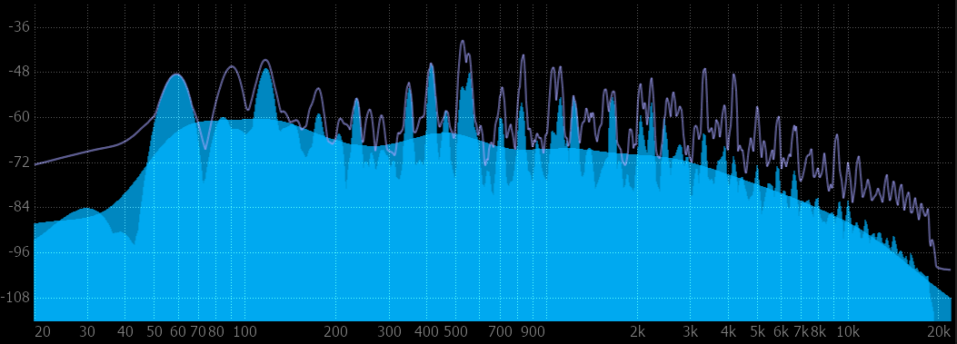
The global principle and purpose of a spectrum analyzer is to transform an incoming signal, which is basically a series of amplitudes taken at successive points in time, into a series of values versus frequency. Transforming an audio signal onto a frequency scale is indeed of great interest in a wide range of tasks, and notably allows to display a global, perceptually meaningful and precise picture of the audio contents.
The display represents the so-called magnitude spectrum of the incoming signal, which is a two-dimensional curve of the magnitudes of the signal taken at frequencies ranging from 0 (DC) to half that of the current sampling rate (or Nyquist frequency in signal processing jargon). This is probably the most commonplace and most easily understood spectrum analyzer visualization, and the place where you should start most of the time when you want to inspect the frequency content of your audio material.
Settings
Block size
Keep in mind that the incoming audio needs to be accumulated in a buffer for a certain amount of time before the data can be computed and the display updated. In contrast with the buffers you probably know from soundcards, this block-processing is not just a computer technicality and only a source of undesirable latency, but an integral part of the process related to the mathematical aspects involved (Time-frequency product uncertainty principle).
As such, it determines both the precision of the analysis and the maximum display rate, and should be adjusted depending on the specifics of your application.
In order to maintain a sufficiently responsive display refresh rate, blocks overlap by 75 %.
The default setting is 8192 samples, which corresponds to a length of roughly 180ms at 44.1kHz sampling rate. This value constitutes a good compromise between precision and responsiveness for most situations. However, if you need to measure a particular frequency with great precision, you should raise the analysis block size. On the other hand, if you need to follow rapid spectrum variations, this value should be lowered.
Transform type
The discrete Fourier transform (DFT) is the traditional method employed to compute the frequency spectrum of a discrete digital signal. DFT can be seen as a series of notch filters centered around frequency bins that are uniformly distributed along the frequency axis, and of constant width.
The quality factor of a resonant filter, commonly denoted as Q, is defined as the ratio of its bandwidth relative to its center frequency. The DFT process is therefore analogous to a variable Q filter-bank: in other words, its frequency resolution is constant across the spectrum. When applied to sliding blocks, this process is called STFT, for Short-term Fourier transform.
Although convenient in terms of computation, this can be seen as less than ideal for many audio applications, for several reasons, the first and foremost being that human perception of frequency is known to be quasi-logarithmic. Logarithmic means that a two-fold increase in frequency translates to a one octave shift, a four-fold increase as a two-octave shift - and not four as this would be the case, were our perception linear in nature.
FLUX:: Analyzer employs both standard DFT and proprietary algorithms that more closely model the human perception. In addition to greatly improving the legibility of the resulting curves, this proprietary transform has the additional benefit of reducing sensitivity to noise in the high-frequency portion of the spectrum especially, and provides more stable readouts.
You can of course switch back to standard DFT by disengaging the Pure spectrum button.
Window type
As previously mentioned, the first step is to split the incoming signal into overlapping blocks. Each block is then multiplied with a so-called window signal prior to the spectrum computation. The purpose of this is to minimize side effects of the block processing, such as introduction of transients at the block boundaries, etc.
The window type to use is set in the Main Main setup setup.
We suggest you leave this setting to the default unless you are quite knowledgeable with these aspects, or in the case you should need to explicitly recreate a specific measurement such as a particular method specified in a standard’s document.
The Wikipedia entry on window functions in the context of signal processing is a good reference if you want to get a more thorough understanding of the subject.
While the windowing process is implemented in the time-domain, it can be also be seen as a smoothing filter in the frequency domain, and as such the choice of window is a compromise between frequency resolution and immunity to artifacts. Skipping the windowing process altogether, which is the same as applying a rectangular window, is not recommended. Although the rectangular window provides the best frequency resolution, it has very poor leakage characteristics.
Ballistics
The curve display update speed is controlled by the ballistics settings.
Release time
The release time determines how fast the main curve falls back to zero. Default is 300ms.
Max release time
The controls the release time of the optional Max curve, which serves to display the medium-to-long term tendency of the magnitude spectrum. Longer times mean curve maxima/peaks will be seen for a longer period.
Default is 50 seconds.
The attack time is zero so the curve displays reacts instantaneously to a rising amplitude.
Averaging
This is a global setting controlled in the Averaging section of the main setup.
Frequency scaling
Scaling controls how the scaling applied to spectrum magnitudes. This is a global setting accessed through the Main Main setup setup panel.
Scaling controls whether frequency-dependent amplitude scaling should be applied. This affects how various standard reference signals register on the display. The default power scaling will result in a signal with spectrum components of constant power registering as a flat curve, whilst amplitude will have the same effect for components of constant amplitude such as pure tones (sine signal).
The table below shows how the curve appearance depending on the type of input signal. 1/f corresponds to a rectilinear slope on the display with both X and Y axis being logarithmic.
| Input signal | Sine | White | Pink noise |
|---|---|---|---|
| Power scaling | 1/f | 1/f | Flat |
| Amplitude scaling | Flat | Flat | 1/f |
For monitoring a mix, it makes most sense to use power scaling, as this is the way our hearing responds. If you need to measure a room’s acoustic response, an outboard unit or a plugin’s frequency response, the system magnitude transfer function is best suited for this purpose and scaling has no effect.
The amplitude scaling setting should therefore really be employed if you need to measure relative amplitude values, such as those of sine test tones at various frequencies. Also, note that plain DFT corresponds to scaling set to amplitude.
The power of a time-signal is proportional to the square of its amplitude, or equivalently, its power in dB is double the amplitude. However, in the case of a spectrum, we are measuring the output of a filter-bank, which reacts very much differently depending on the type of input signal, so the simple previous formula doesn’t apply anymore.
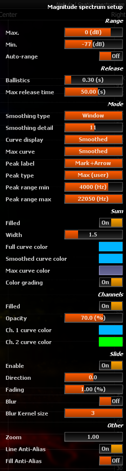
Display range
Display range can be switched from a fixed reference interval to one that automatically adjusts to the current range of spectrum magnitude values. The latter is useful as a set and forget setting and works well to display the most vertical detail, at the expense of losing the ability to visually compare the current values to a reference level.
dB Min / dB Max
Sets the minimum and maximum magnitude to display, in decibels. This is visible the range of the display that is taken into account when auto-range is off.
Default range is -18dB (min) to -114dB (max).
Range mode
Default is Manual.
Manual
Uses a fixed range as specified by the above settings.
Auto
When engaged, auto-range continuously adjusts the display to the current range of the data.
A slight envelope is applied to the auto-range values in order to improve legibility, avoiding the display to follow every minor change. Peaks are always registered however, as these provide valuable information that should not be missed.
Compressed
The range is defined by dB Min/Max values, and the Y-axis is also compressed in the lower range. This can bring out peaks and valleys in the spectrum to better visualize resonant frequencies and such.
Compressed | Auto
Combines Compressed and Auto modes.
Summation
These settings allow you to modify the appearance of the curves in channel sum mode.
Filled
Toggles whether the main curve is drawn as a solid-color fill or a plain line.
Default is on.
Width
Thickness of the pen used to draw the curve lines, in pixels.
Default is 1.0.
This setting also affects individual curves when channel sum mode is disabled.
Full curve color
Color of the pen used to draw the main, full-detail, unsmoothed curve.
Smoothed curve color
Color of the pen used to draw the smoothed curve.
Max curve color
Color of the pen used to draw the max curve.
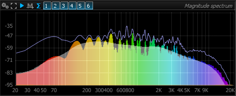
Color grading
Applies an optional frequency-dependent coloring to the main channel-sum curve.
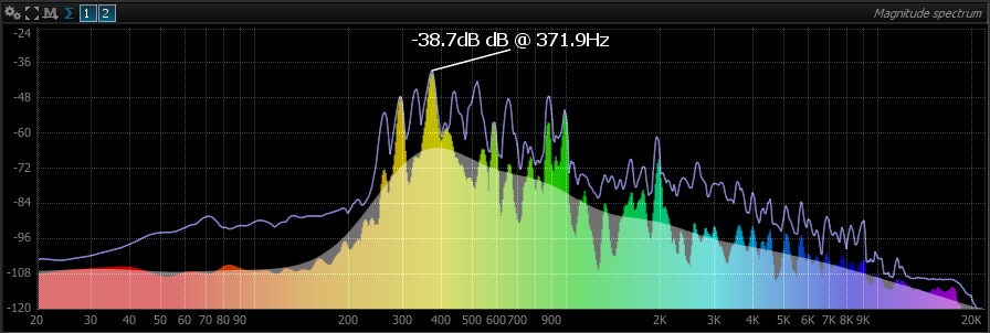
Magnitude spectrum with color grading enabled
When enabled, any of the above fixed color settings are overridden.
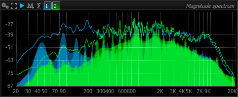
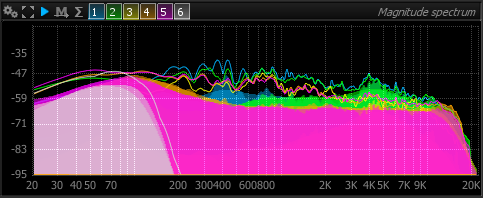
Channels
This group of settings controls the appearance of curves when channel sum mode is disabled. There is one Ch.N curve color setting per channel, so you can fine-tune the color scheme employed if you wish to do so.
Filled
Controls whether channel curves are drawn as a solid color fill or a plain line.
Opacity
Controls the opacity of the fill when Filled is enabled. 100% gives a fully opaque fill, lowering this value makes the curve fill more transparent.
Channel curve color
This setting controls the color of the curve corresponding to the n
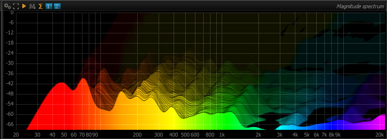
Slide (Real Time waterfall)
Enable
Enable/disable the slide mode.
Direction
Define the sliding Direction. From -5 to 5.
Default is 0.
Fading
Controls display persistence, i.e. the “fade to black” amount for a frame. Lowering this value retains past particles longer, whereas increasing this make them disappear faster.
Blur
Enable / Disable sliding blur.
Blur Kernel Size
Controls the radius of the blur effect applied to past particles. Particles are “smeared” more and more as they become older, depending on this setting. Naturally, a bigger value increases the smearing, at the expense of processing power.
Choosing the value for this setting is really matter of taste, although please keep in mind values that above 5 will require a sufficiently powerful graphics card in order to maintain a responsive display.
Zoom
This setting allows to check and change the current X-axis zoom level.
Default is 1.0, which corresponds to the whole frequency spectrum. Zooming with the mouse is the preferred way, as it offers more control.