Transfer function
Introduction
The transfer function of a system measures its frequency response, which is expressed in terms of magnitude and phase response. The transfer function measures the way the system affects the magnitude and phase of an incoming signal at different frequencies, and is essentially a ratio of output versus input spectra.
Practical uses of this are numerous: determining the curve of an equalizer, determining what frequencies are emphasized by an outboard device, measuring a room’s acoustic response, etc.
The transfer function assumes the system meets the following conditions: linearity
time-invariance
Linearity notably implies the system is free of distortion, and time-invariance that its characteristics do not change in time.
Failing to meet these requirements will lead to unpredictable results.
In practice, the transfer function is considered an adequate measurement technique for most real-world systems, except for devices exhibiting highly non-linear behaviour such as compressors and distortion effects, and time-modulation based effects such as chorus and flanger.
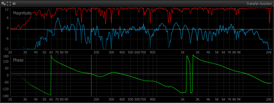
Transfer function magnitude
The transfer function magnitude displays the gain versus frequency curve of the system under test. A pass-through obviously results in a flat horizontal line centered on 0dB. This line represents the ideal curve one would be able to achieve if all the systems defects could be compensated for, and that serves as a reference target when doing room correction.
Transfer function coherence
Coherence is a normalized - that is comprised between zero and one - measure of the confidence of the transfer function at a specific frequency.
In other words it describes how trustworthy the transfer function is at the corresponding frequency.
Coherence at a particular frequency indicates whether the system can accurately be described as linear gain and phase shift or not.
Interpretation and uses
Low coherence most often indicate a bad measurement, so you should look for possible causes and correct them before starting again.
Typical culprits include a noisy device, presence of distortion, channel crosstalk, acoustical noise such as cooling fans, people talking, handling noise, bad isolation from the outside, etc. Low coherence also manifests when delay is improperly compensated for.
While maximizing coherence is desirable, in most cases, it will most likely be impossible to attain a flat curve approaching unity at all frequencies, except in an anechoic chamber or very ‘dead’ sounding room with minimal reflections.
Reverberation, as well as mismatched transducers, tends to give lower coherence, as the signal arriving at the microphone position is really the sum of several time-delayed version of the source.
Sometimes it will be impossible to get good overall coherence, and the magnitude and phase curves will therefore be less precise, stable and smooth. This does not mean you cannot attempt extract any information from those. As always, use your judgment and knowledge of the specific system to decide which assumptions seem reasonable.
Display
By default, the transparency of the main magnitude curve is also modulated with the coherence values, which increases readability by effectively dimming untrustworthy curve portions. In addition to controls and settings identical to those of the spectrum magnitude curve, you can toggle the coherence curve on and off with the ‘Enable’ switch under ‘Coherence’ in the settings.
Transfer function phase
Phase information is sometimes overlooked, and indeed it is less straightforward to understand and interpret than magnitude. Altering the phase of a signal can range from subtle to dramatic, and phase distortion can lead to temporal smearing of the audio, loss of spatial information, and other nuisances.
The transfer function phase curve displays the phase difference between output and input of the system at different frequencies, in degrees, ranging from -180 to 180.
FLUX:: Analyzer employs several smoothing algorithms custom designed for phase curve smoothing, as explained in the section about Phase setup.
Due to the definition of phase itself and the means of computing it, the curve is generally more sensitive to extraneous noise, distortion and time-varying conditions.
Even more so than with the magnitude curve, a precisely compensated delay is critical to accurate phase computation. ∏˜
In very reverberant environments, the phase curve will be very chaotic.
This is inevitable and a direct consequence of the complex nature of the system, and not a limitation of the instrument.
We advise to use Pure spectrum analysis mode which mitigates phase computation inaccuracies compared to plain FFT. :::
Setup
Time averaging is on by default as the goal here is to provide the most stable display, and to eliminate any variations of the signal in time.
Frequency smoothing can be useful to smooth out irregularities and get a general picture of the curve. It is advised to use this function sparingly though, as it can change values by a large proportion, and obscure potential problems with either the actual system being measured, or the measurement setup itself.
A combination of time averaging and frequency smoothing is most often required to obtain readable results in real-world scenarios, especially with large rooms and outdoors.
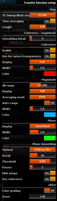
Main
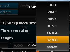
TF/Sweep Block size
Block size used for the transfer function and the snapshot done with sweep. The default is 32768, which is appropriate for most cases.
Increasing this value gives better frequency resolution, at the expense of CPU load. Lower values can be employed if you’re only interested in the overall response of the analyzed system.
Time averaging
Toggles time averaging on and off. Default is on, which in most cases is necessary to provide a stable display readout.
Length
This setting determines the number of blocks taken into account to compute the averaged transfer function. Increasing this value will give a smoother readout, but the display will react more slowly to any input variations, and CPU load will be higher.
The default is 32.
Coherence / magnitude
Smoothing detail
Sets the amount of detail present on the smoothed magnitude and coherence curves. This number is roughly the maximum number of valleys and peaks that will remain after smoothing. A low value of around 10 is good for getting a global and uncluttered picture of a room’s frequency response.
Relying on smoothed curves altogether should be avoided, as smoothing can mask-out essential information such as room modes, which materialize as sharp peaks and dips in the transfer function magnitude curve.
We strongly recommend basing your judgment on both raw and smoothed curves even when the raw curve is very noisy.
Coherence
Enable
Toggles the display of the coherence curve on or off. With multiple snapshots, the display can rapidly become crowded, and in that case hiding the coherence curves will improve legibility. In the general case however, we recommend leaving this enabled as coherence represents important information which should not be overlooked.
Use for curves transparency
Allows to use the coherence values to define Magnitude and Phase curves transparency.
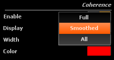
Display
Toggles between one of three modes:
- Full : main unsmoothed coherence curve.
- Smoothed: smoothed coherence only.
- All: both.
Width
Size of the pen used to draw the coherence curve.
Color
Color of the pen used to draw the coherence curve.
Magnitude
Range
Minimum and maximum values to which the display is clamped, in decibels.
Display
Toggles between various combinations of raw and smoothed magnitude curve display.
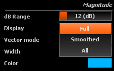
- Full : main unsmoothed magnitude curve.
- Smoothed: smoothed magnitude only.
- All: both.
Keep in mind the smoothing process can filter out a lot of information, so relying solely on the smoothed curve should be avoided.
Averaging mode
Choose he averaging mode of the transfer function magnitude.
Vectorial mode computes the average sum of magnitudes and magnitudes multiplied by coherence. In vectorial mode, the averaged magnitude is therefore and indication of the perceived magnitude spectrum, i.e. the sum of the direct path and diffuse field signals.
Default is RMS
Auto-Range
Toggles auto-range on and off. When enabled, the display range automatically follows that of the transfer function magnitude curves, which is useful for hands-free operation, for example. Default is off.
Width
Size of the pen used to draw the magnitude curve.
Color
Color of the pen used to draw the magnitude curve.
Phase
Phase curve specificities
You will notice the phase curve is generally very sensitive to spurious noise and interference, and that in general it requires a bit of work on your part in order to read and interpret it. Outside of the studio, in noisy places such as a live venue, phase smoothing is almost always mandatory in order to get a readable curve. It is important to understand that smoothing destroys information in order to achieve this, so you should always double-check what you see on the smoothed curve against the original, raw data.
The algorithms employed here are specific to phase, and have more options than the regular smoothing employed for spectrum magnitude, transfer function magnitude and coherence, in case you wish to fine-tune their behaviour.
Display
Toggles between the various phase curve display modes:
- Full: raw phase only.
- Smoothed: smoothed phase only.
- All: both.
Width
Size of the pen used to draw the phase curve.
Color
Color of the pen used to draw the phase curve.
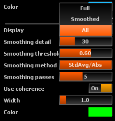
Phase Smoothing
Method
Please refer to Phase smoothing methods.
Detail
Adjusts the overall level of detail that remains after smoothing, in percent. Do not set this too low or you might miss out important information such as phase shifts at critical frequencies such as those associated with loudspeaker crossover networks.
Values around 30 are appropriated in the general case.
Threshold
Amount of relative local phase variation that is allowed to pass through. Raising this filters out local phase curve detail, such as noise. Setting it to one suppresses all detail, whilst setting it to zero leaves the curve untouched.
0.60 is a good starting point.
Passes
Sets the number of smoothing algorithm iterations. You can apply the smoothing process several times in order to get better results whilst still retaining local detail. Increasing this value requires more CPU processing power, so it is advised to lower this value if you find your computer cannot cope with the load. Default is 5.
Hide jumps
When enabled, the portion of the curve that corresponds to a phase rotation is not displayed.
Uses coherence
When enabled, frequency regions of the phase curve with low coherence are applied more smoothing. Conversely, regions with coherence close to one are applied little or no smoothing.
Low-coherence regions are caused by low signal-to-noise ratio, multiple paths, etc. which cannot be accurately described in terms of a simple gain and a phase shift anyway, so it makes sense to suppress excess detail in these regions to improve the curve’s general readability.
Method
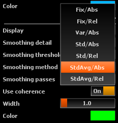
Available phase smoothing algorithms.
The general principle is that for each curve pixel, the algorithm determines the amount of smoothing applied in its neighboring region, based on a threshold determined from other pixels in the region. The smoothing therefore adapts to the curve content, applying more smoothing in noisy regions.
StdAvg/Abs was determined to be method giving the best results in the general case, and is set as default. You might still want to experiment with other algorithms, especially if you have a slow computer.
Fix/Abs
This is the simplest and least CPU-intensive phase smoothing algorithm. Smoothing uses surrounding pixels below an absolute threshold.
In practice, this means curve regions with large variations are applied stronger smoothing.
Fix/Rel
Same as above, using a relative threshold.
Var/Abs
A variant of first algorithm.
Std/Abs
The threshold is determined from the pixels standard deviation, which is a statistical measure of data variation.
Std/Rel
Same as above, using a relative threshold.
StdAvg/Abs
Combination of above methods, using absolute threshold.
StdAvg/Rel
Combination of above methods, using relative threshold.
Please keep in mind the smoothing process is purely a visual aid, and is not intended to compensate for an inadequate measurement setup. In short: always rely on your ears and scientific knowledge first !
Other
Color grading
Apply frequency-dependent coloring to the curve. Default is off.
Zoom
Curve zoom ratio slider.