Exploring the Fourier Transform

This chapter provides an easy-to-understand introduction to the Fourier Transform and its derivatives. It explains the technology behind a spectrum analyzer, which will help sound engineers understand the capabilities and limitations of their tools.

Introduction to the Fourier Transform

Fourier and the Dual Representation of Signals

Sound phenomena can be described as variations in air pressure over time. We typically capture these variations using transducers called microphones that convert air pressure variations into voltage variations.

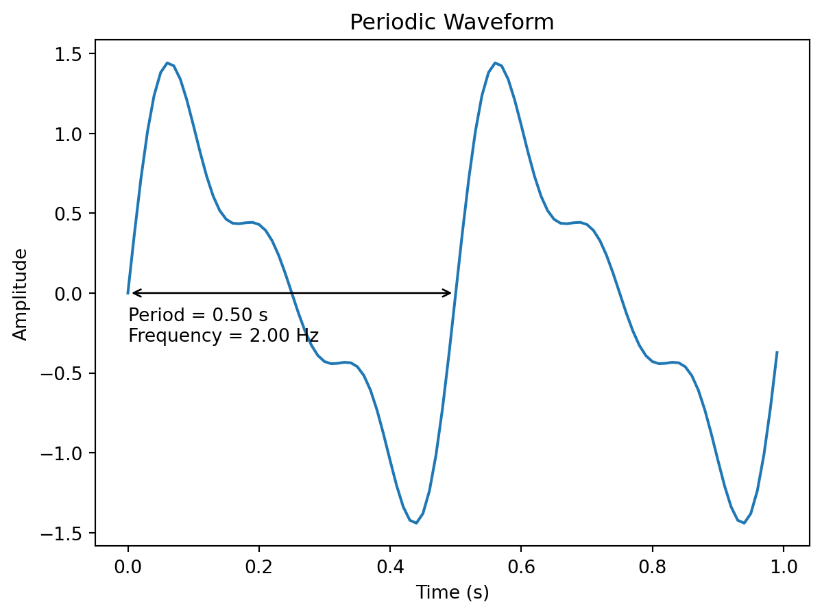
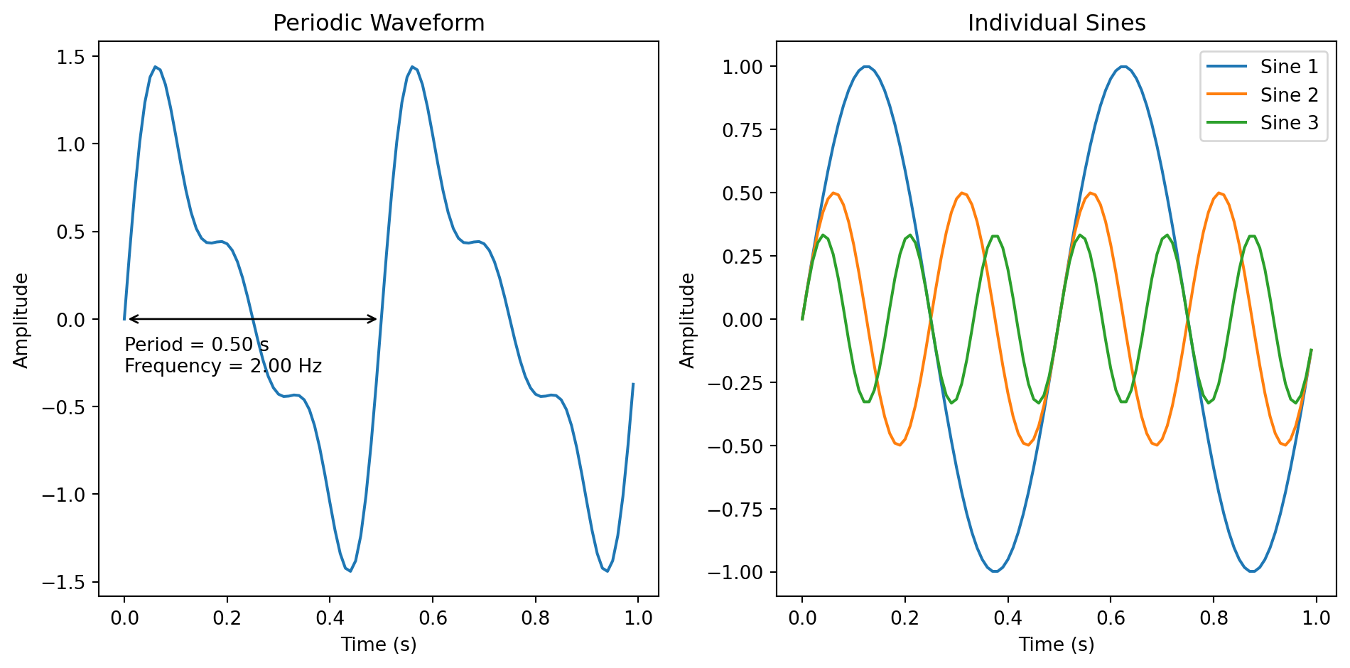
Joseph Fourier, a French mathematician and physicist who lived from 1768 to 1830, first proposed that any periodic signal can be expressed as a sum of pure tones.

A periodic signal is any signal that has a constant and repeating pattern over time. The length of the pattern is called the period, and the number of times the pattern repeats over one second is the fundamental frequency of the signal. Periodic signals usually exhibit harmonics. Harmonics are other frequencies existing in a periodic signal that are multiples of the fundamental frequency.

Pure tones correspond to particular periodic signals, which are also known as sinusoids. They have the unique property of having only a fundamental frequency and no harmonics. Due to this property, we can understand that a more complex periodic signal is the sum of multiple pure tones having frequencies and amplitudes that match those of the harmonics and the pure tone of the studied signal. This is the principle of the Fourier Series.

The Fourier series only applies to periodic signals. Most real-world signals, however, are not. To overcome this problem, Fourier extended the Fourier Series to the Fourier Transform, which can be applied to any signal.

The Fourier Transform can be thought of as a band-pass filter bank where the output amplitude of each band-pass indicates the presence of sound energy in a certain frequency range.

The Fourier Transform is the foundation of many spectral analyses.

Fourier Transform in digital systems

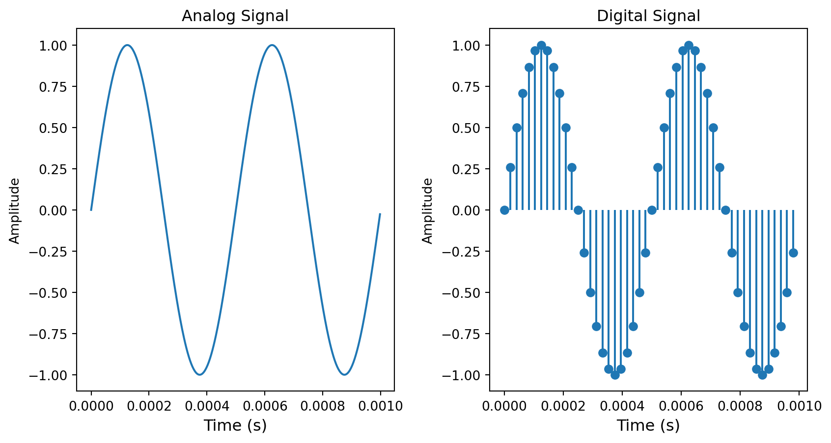
So far, we have considered audio signals in the analog domain. The analog domain is characterized by time continuity, meaning that the value of an audio signal can be determined at any instant.

Computers cannot process analog signals because they require an unlimited amount of processing power and memory for any time span. To overcome this limitation, we sample analog signals, meaning that we take a value at regular intervals, transforming a continuous function into a discrete set of points. The frequency at which we take a value is called the sampling rate, and it also defines the maximum frequency that our digital system can correctly sample. According to the Shannon-Nyquist theorem, we must have a sampling rate at least twice as fast as the highest frequency in the signal we want to sample. Since it is generally accepted that human hearing does not detect sounds above 20 kHz, the typical sampling rate for audio signals is often around 40 kHz. This upper frequency limit is known as the Nyquist Frequency.

Since a digital system processes discrete audio signals, we must modify the Fourier Transform into a computable algorithm.

The definition of the Fourier Transform poses two significant limitations in the context of digital systems.

1. The Fourier Transform tries to identify any possible frequencies inside a signal. We need to define a limited range of frequencies to be able to perform this operation in a digital domain.
2. The Fourier transform also assumes that the signal is known throughout its lifetime. This restriction limits its use to offline analysis, making it impossible to apply in real-time.

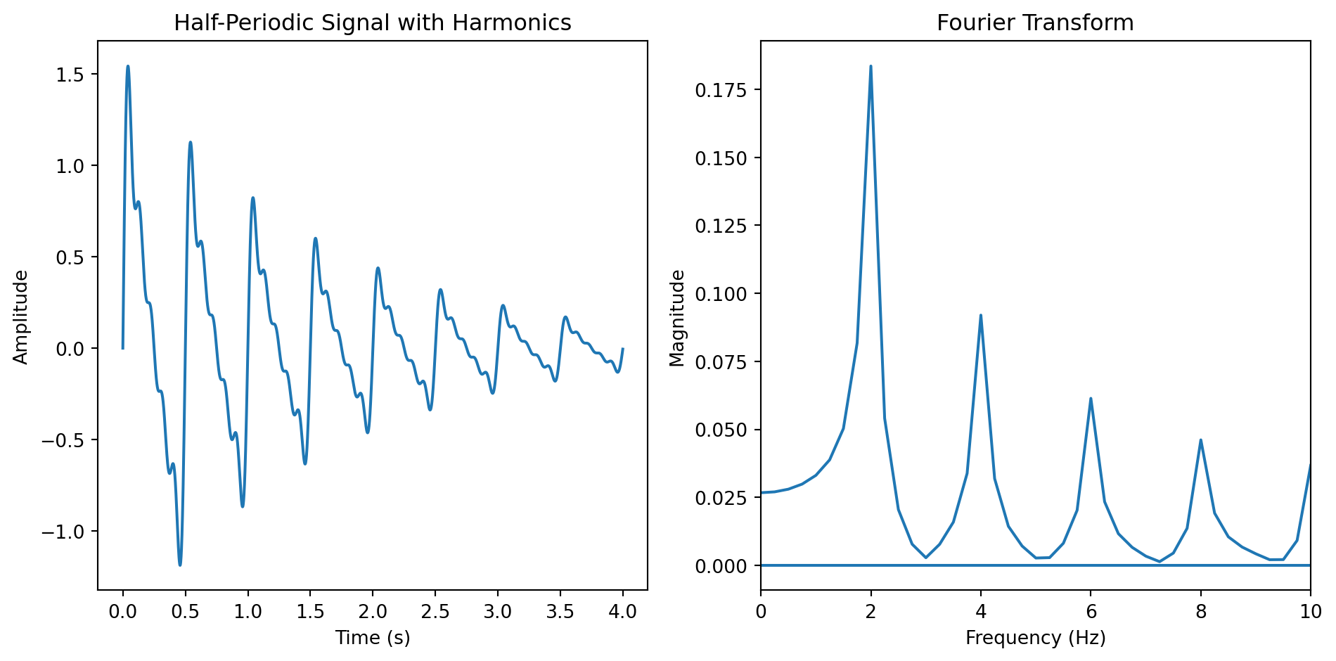
The Discrete Fourier Transform was introduced to address the first problem. This method takes a completely known input signal and finds all frequencies with a period that is a multiple of the signal’s length, up to the Nyquist frequency.

To address both problems, we use the Short-Time Discrete Fourier Transform (STDFT). This method allows us to analyze an incoming audio stream in several chunks, or buffers, rather than the whole audio file. We then follow the same process as for the discrete Fourier transform. Usually, the length of each buffer is referred to as the window analysis length. The STDFT outputs what we call frequency bins. Each frequency bin can be interpreted as a band-pass filter with a width equal to the inverse of the window analysis length.

The Fast Fourier Transform (FFT) is a specialized algorithm that we often use to calculate the Short-Time Discrete Fourier Transform. It has the particular property of being particularly efficient for buffer sizes that are powers of 2.

The uncertainty principle

When analyzing the content of an audio signal using an FFT, the length of the window analysis is a very important parameter to set up correctly.

A larger window increases the precision of our spectral analysis by reducing the step between each frequency searched in our audio signal. It also improves the low-end resolution in the context of audio signals. However, a larger window requires more samples from the input signal, making the analysis less responsive to rapid changes in the signal.

In simple terms, we can’t have good frequency and time resolutions at the same time.

A first summarize

To get insight into a signal’s spectrum, one needs to use the Fourier Transform. In the digital world, we use the Fast Fourier Transform, which is an optimized implementation of the Short-Time Fourier Transform. It can be performed in real-time. An FFT needs a window size, which corresponds to the number of samples taken into account for the spectrum analysis. A larger window size leads to more resolution in the low-end of the audio spectrum, while a shorter window size gives a better time reactivity. The FFT algorithm can have both a very good time and frequency resolution.

Understanding a Real-Time Spectrum Analyzer

Real-time spectrum analyzers use FFT, or derivative strategies, to analyze incoming audio streams. Since such algorithms, as seen above, have limited frequency resolution, some inherent limitations are observed. Therefore, it is crucial for users to recognize and understand these constraints in order to accurately interpret the presented data.

Why do some pure tones seem wider than others?

To demonstrate the MiRA real-time spectrum analyzer, we will conduct a straightforward use case by transmitting various pure tones and analyzing the results. To begin, let’s adjust the main settings. The window size will be 1024, and the window shape will be rectangular.

Caution

Unless you are absolutely certain of what you are doing, you should never change the default settings.

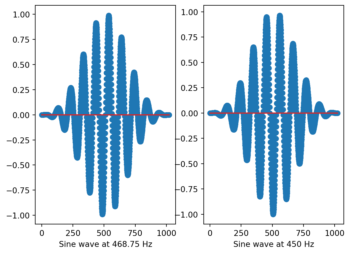
Now, we will set a sine wave generator to 468.75 Hz and observe the result. We observe a frequency spike that is quite narrow. However, if we slightly alter the frequency of our generator, we will observe a significantly different outcome.

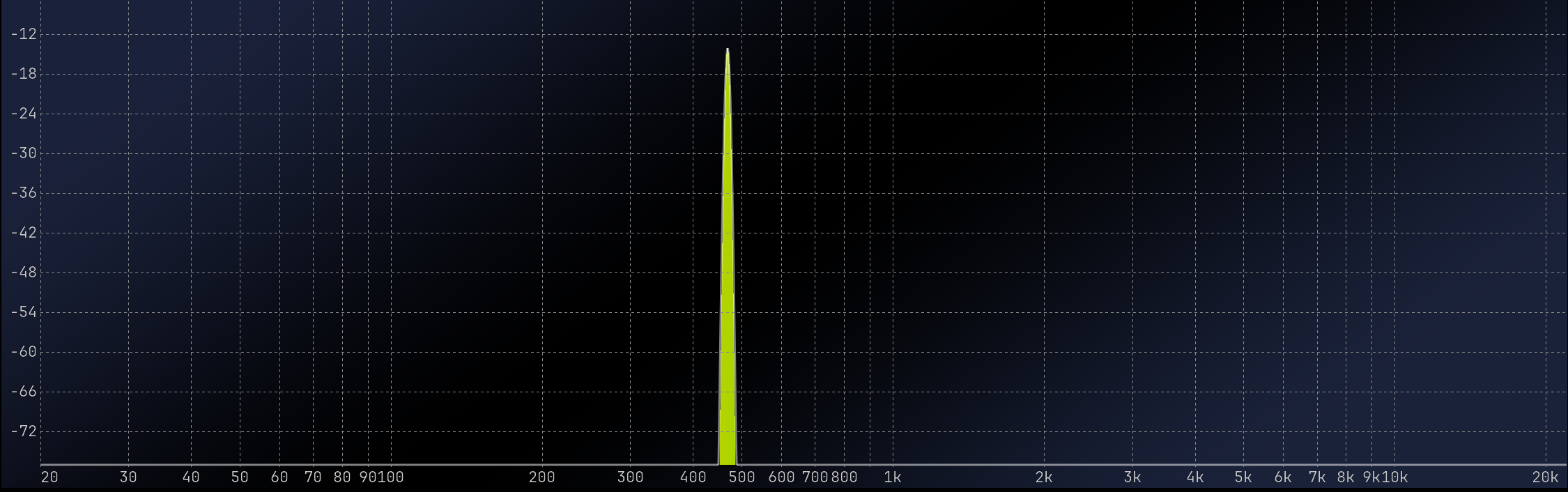
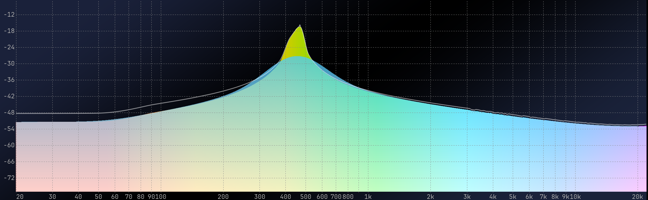
At 450 Hz, the visualization generates a wide frequency peak with a high noise floor. Let’s look at the two waveforms over a 1024-sample period to see what’s happening.

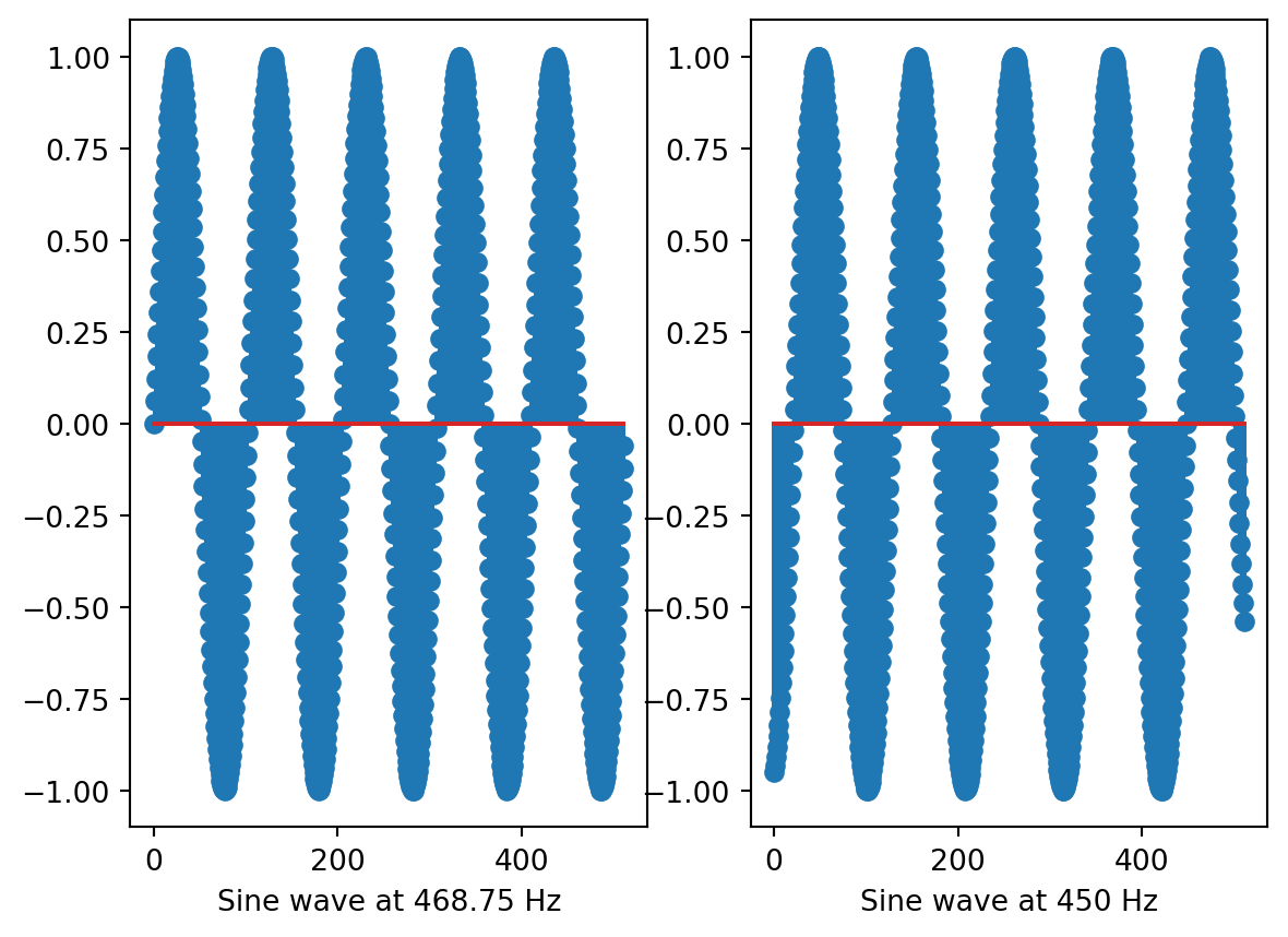
The left plot displays a waveform that precisely matches the length of the window size. In contrast, the right plot reveals a discontinuity. The FFT algorithm hears the discontinuity as a click, leading to the aforementioned issues in the resulting plot.

This phenomenon can be understood in a similar way to what occurs in an audio editor when attempting to edit without applying any fade-in or fade-out effects. You can hear clicks happening too!

Windowing functions as fade in/fade-out

Windowing functions apply amplitude factors over a given time interval to smooth out discontinuities that may appear during the FFT computation.

Here is a visual representation of various types of windowing functions:

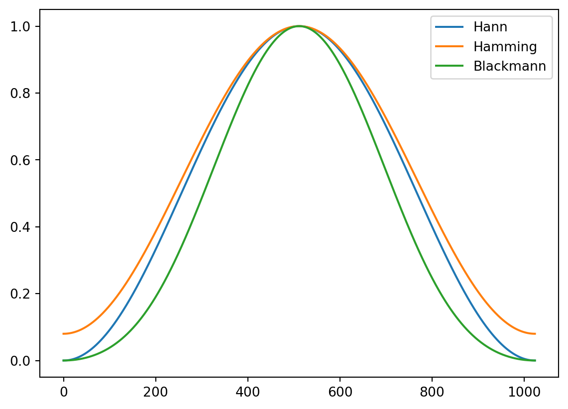
The default window shape in MiRA is Blackmann. If we apply this windowing function to our two sine waves, here is what they look like:

Now, you can see that the buffer’s extremity has faded to zero, thus removing the discontinuity.

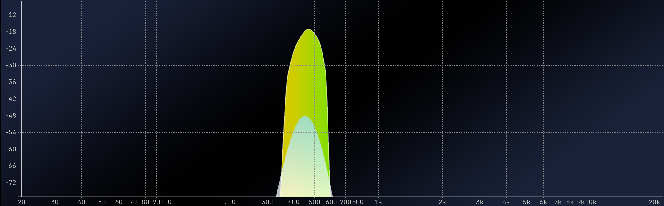
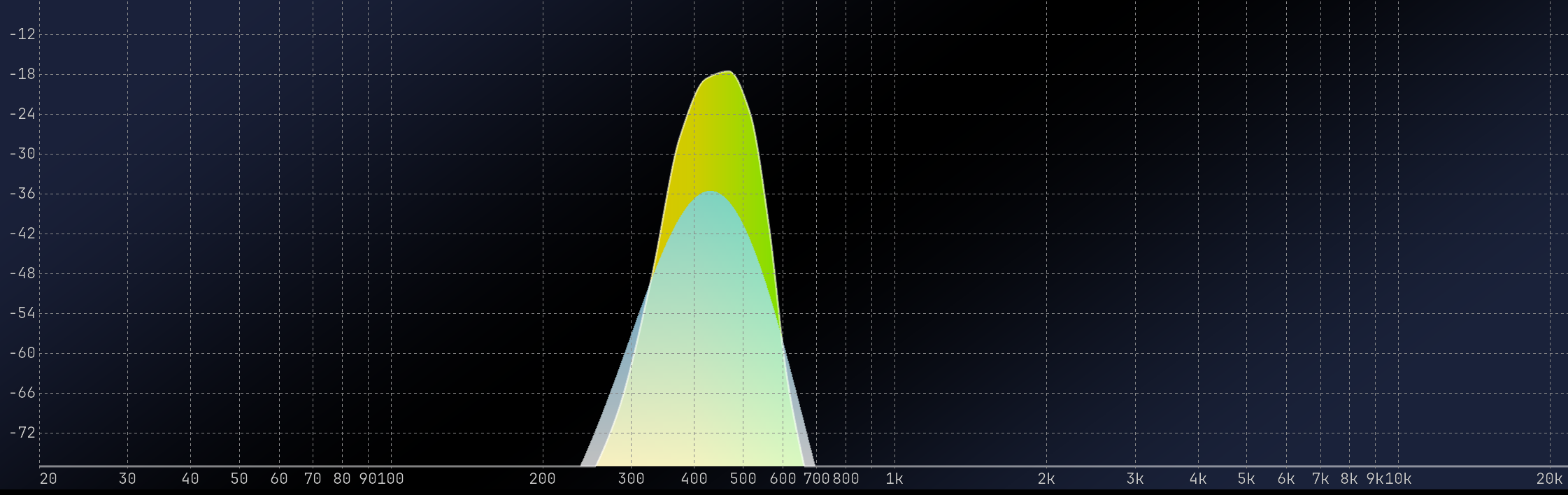
It’s clear that our windowed sine wave at 450 Hz has significantly better results, although there is a slight decrease in accuracy for the 468.75 Hz sine wave. It is strongly advised that you consistently use a windowing function, as there is no justification for a signal to display frequencies that are only multiples of the FFT size.

To achieve a higher degree of precision in frequency resolution, we can extend the analysis period. In MiRA, the default value of 8192 generally strikes a balance between frequency resolution and time accuracy.

Limitations of the Fast Fourier Transform

The Fast Fourier Transform is a valuable tool, but it has some limitations. One of the main ones is that it samples the frequency domain with a constant frequency step, which means that our logarithmic perception of frequency results in a higher resolution in the high-end of the spectrum and a lower resolution in the low-end. For example, the default window length of MiRA is 8192 samples, giving a frequency step of about 5 Hz. While this resolution is acceptable for the low end of the spectrum, it provides so much information on the high end that it makes it difficult to understand what is happening. Also, computing so many points requires a significant amount of CPU resources.

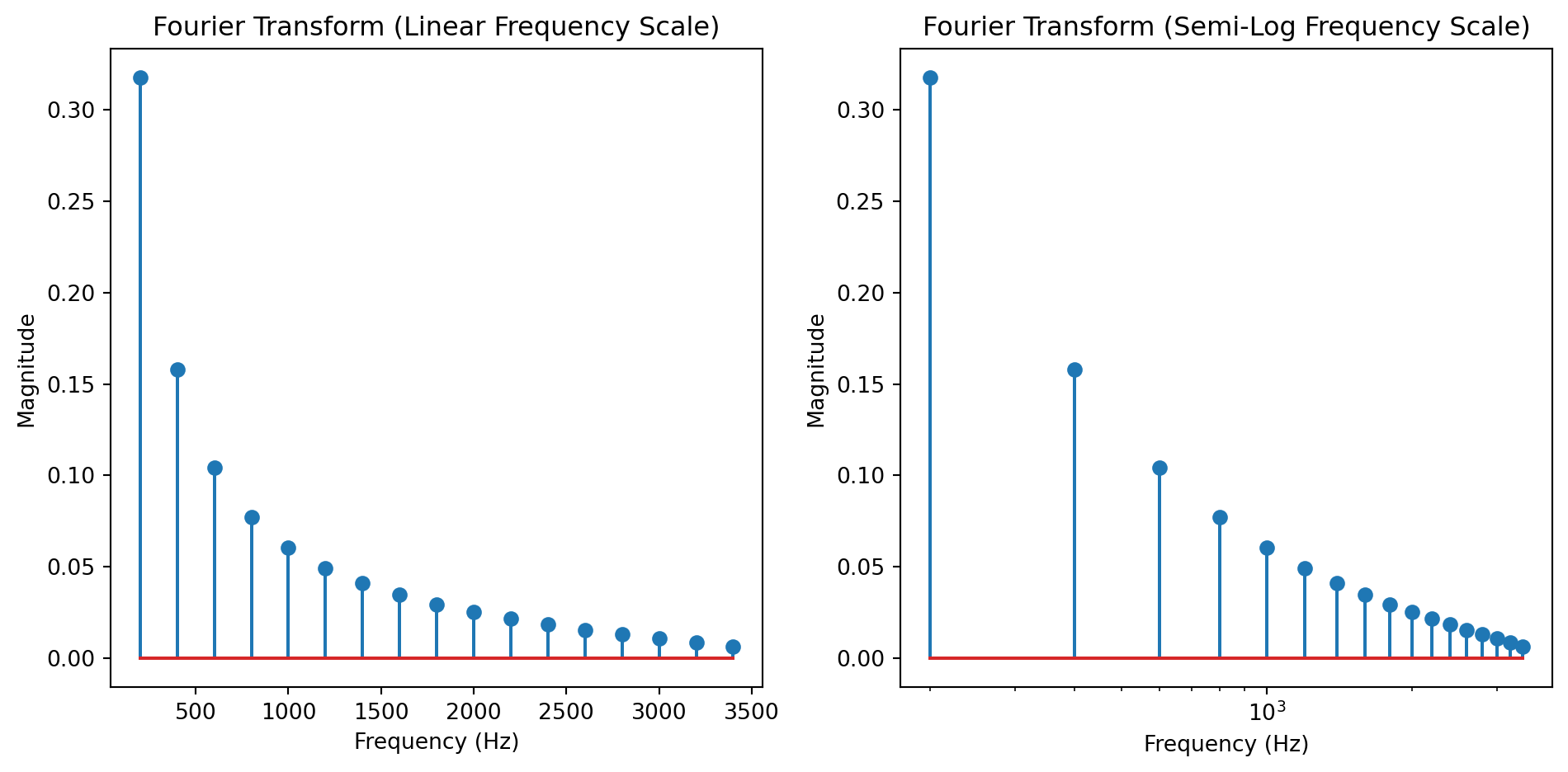
In the spectrum above, which represents a 200 Hz sawtooth, you can see that, when displayed logarithmically, its resolution is poorer in the low-frequency range. With richer signals, finer resolution in the high-frequency range can appear as noise. The measure itself is not noisy, but the greater point density can make plots challenging to read.

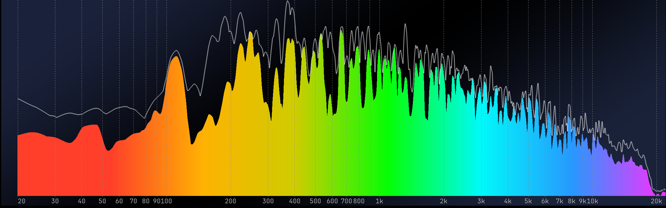
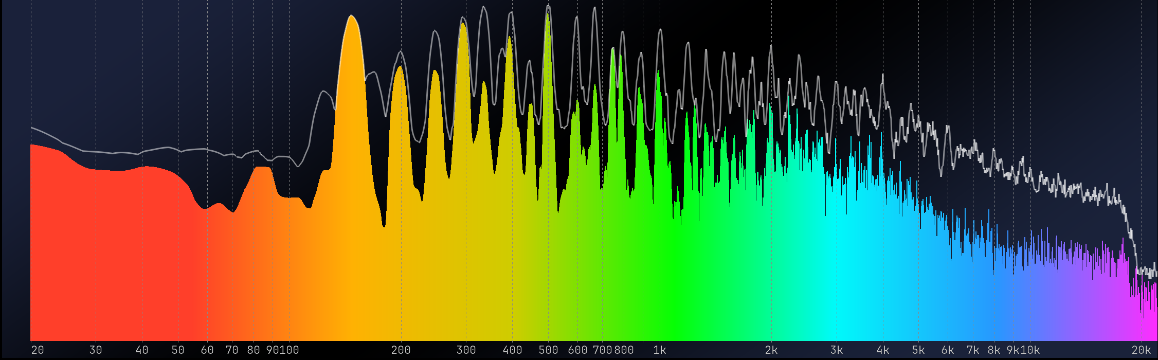
Ideally, we would like a Fourier Transform that corresponds to our logarithmic sound perception. Two implementations in MiRA:: can address this problem: the Variable-Q transform and the Adaptive Resolution Transform.

MiRA Propriatory Transforms

This section describes the two proprietary FLUX:: transforms: the variable-Q transform and ART. It details their advantages over plain FFT in the context of audio analysis, as well as their main use cases.

The Variable-Q Transform

The FLUX:: Variable-Q Transform (VQT) is an algorithm that matches auditory perception. As a reminder, our perception of frequency is logarithmic. For example, if we perceive a difference of one octave between two notes, the higher note has a frequency that is twice as high. The idea behind the VQT is to maintain a constant number of frequency bins per octave, thus maintaining a constant level of resolution with respect to our perception.

Such a strategy has several advantages:

• Although the variable-Q transform requires slightly more computing power than a simple FFT, it generates less data, making it much more efficient to use in MiRA.
• With its default window size of 8128 samples, the VQT provides a good resolution in both the low-end and high-end.

The Variable-Q Transform is the cornerstone of MiRA’s real-time frequency analysis, since it is, by default, the engine of each scope displaying frequency information.

ART (Adaptative Resolution Transform)

The FLUX:: ART algorithm aims to solve two problems:

• Uneven resolution in the FFT when considering a logarithmic scale.
• The difficulty of obtaining good temporal and frequency resolutions.

The idea of ART is to use multiple FFTs of different sizes, depending on the octave under consideration. Higher octaves can use very short FFT sizes, which gives them excellent time resolution. At the same time, this keeps a good frequency resolution for the part of the spectrum we are considering. For lower octaves, however, the FFT size increases in order to maintain good frequency resolution.

When combined, all of this data provides a fairly consistent distribution of points, taking into account our logarithmic perception, while remaining quite sensitive to very fast information such as transient.

Thus, ART is the default algorithm for our transfer function scope.