Sessions and Captures System

Introduction

MiRA has a very complete system for managing all the measurements done by the user.

Inside the application, a measurement is called a capture. A capture contains the channel’s spectrum, transfer function and impulse response.

Captures are organized per session. Each session is materialized by a .fcap file inside the following folders:

~/Library/Application Support/FLUX/MiRA/Captures on macOS
C:\User\/...\AppData\Local\FLUX\Captures on Windows.

A session can serve multiple purposes. It can represent the ments of the sound system of a venue or of a specific audio equipment. It can also serve to store calibration files or target curves.

Note

MiRA can import a wide variety of calibration and measurement files from other manufacturers, including, amongst others, Behringer, Beyerdynamic, Dayton, Earthworks, Isemcon, Neumann, Sonarworks mics, and Smaart and REW text exports.

For system tuning, the main workflow strategy of MiRA is to allow very quick system measurement while giving you all the tools to work and recompute offline.

To perform an on-site measurement, you can use pink noise to calibrate the delay finder algorithm, then use a few sweeps to measure what you need to (heads, subs, front-fields, etc.). Note that MiRA has its own signal generator to ease this process.

Once the captures are acquired, MiRA can recompute delays, average, acoustic sums and so on without having to feed any measurement signals through the sound system again

Performing a capture - quick start

I/O setup

The first step of any capture process is to make sure that the I/O is correctly configured. Go to the IO menu, by reaching either the info header, or to the top menu Mira>IO settings on macOS, or Files>IO settings on Windows.

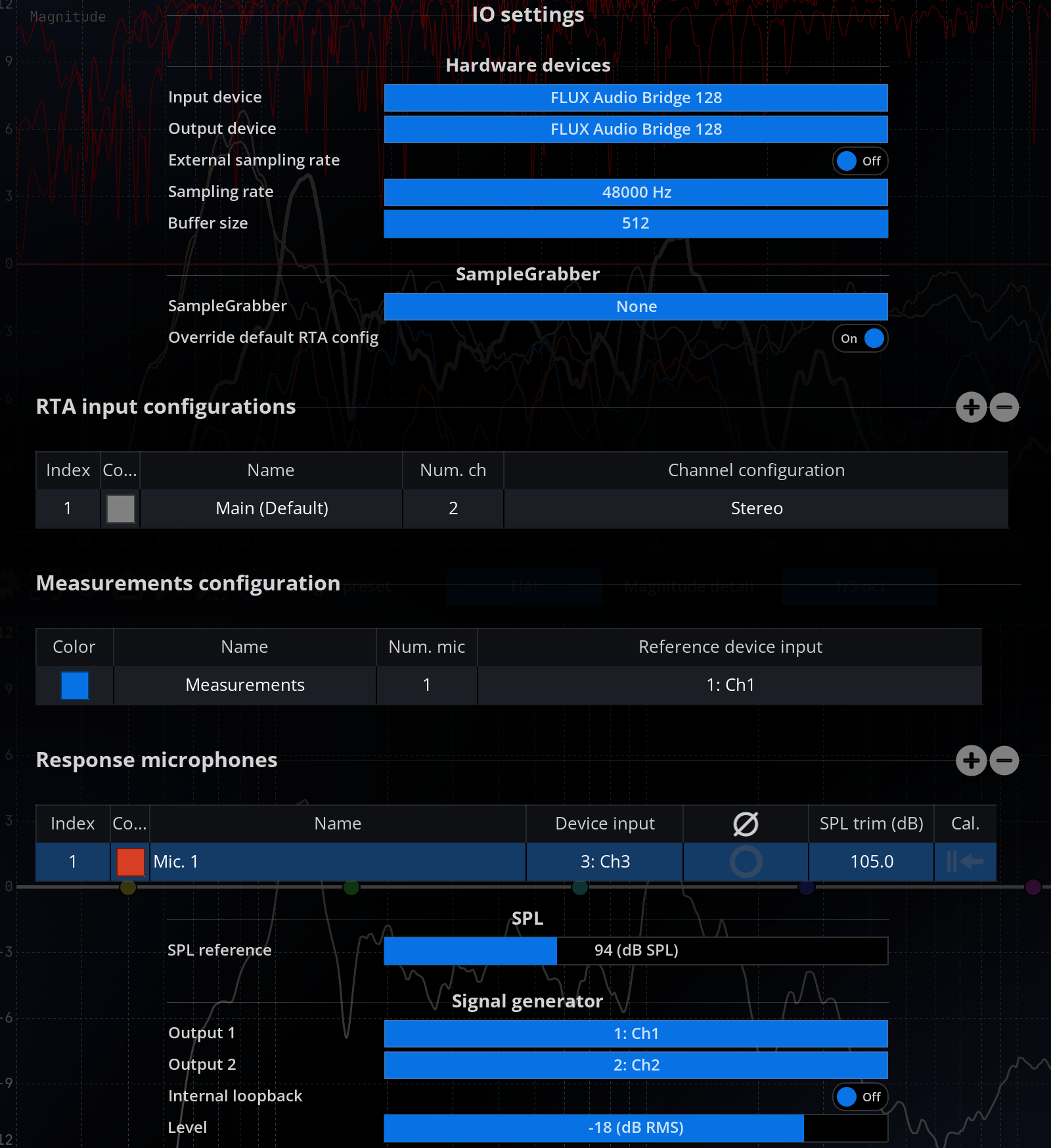
Make sure to select the correct input and output of your audio interface. You should then configure the different input channels of the capture system. In this example, the number of Response microphones is set to one. In the measurement table, the reference device input (transfer function reference) is set to input channel 1. In the Response microphone table, the input of the first response microphone is set to input channel 3.

With these settings, our measurement will be fed to input channel 3.

We also need to ensure the signal generator is correctly patched. In our example, we want the signal generator to output on channels 1 and 2. The same signal is sent to both channels as this simply makes the next part of the routing easier. Output 1 of our audio interface is looped back to input 1. Output 2 goes to the system under test, and the output of the system goes to input 3 of our audio interface.

At this point, our routing setup is ready.

Creating a session

The very first step is to create a new session to store our captures. Simply click on the “new session” button. A popup appears which is used to give the session a name. Name it accordingly and press OK.

Checking for delay offset

It is absolutely crucial to make sure that all your microphone inputs are properly aligned with the reference signal. In MiRA, the recommended method for this is to set the signal generator to a pink noise and start it. If our previous routing is correct, we should now see some time offset appearing in the \(\delta\) column of the system.

You can compensate for these delays by clicking on the button.

Acquiring the capture

It is of first importance to understand that there are two main ways to create captures:

You can send any signal into the system to measure, then create a capture once the curves have stabilized.
You can create an automated capture using a swept tone signal or a pink noise.

To use an automated pink noise to perform the measurement in MiRA, simply click on the icon; click on the icon for an automated sweep tone measurement. MiRA will then ask you to name each capture.

Repeat the process for each measurement that you wish to create (different loudspeakers, heads, subs, front field, etc.).

Capture a computed curve

If you want to capture only an average curve, you can use the action “New computed capture” in the “Capture” menu, or the shortcut Alt + Shift + Space. This will create a new capture with the current state of the computed curve, without capturing the individual microphone curves.

Sequential captures

In order to help perform several measures in a row, MiRA provides a way to create sequential captures. To do so, use the action “New sequential captures” in the “Capture” menu, or the shortcut Ctrl + Alt + Shift + P. A dialog box will appear asking you to define the number of captures, the waiting time between each capture, and the signal type.

Capturing online and processing offline

In the previous section, we have seen that many parameters are related to the different input channels. It is very important to understand that none of those are permanently bound to the measure itself. You can always modify the applied delay, capture and target curves, microphone pairing and gain afterwards.

The computation curve itself is automatically regenerated based on any modifications made to the captures. The main idea is, as stated above, to capture online and to process offline. In other words, most of the system tuning tasks can be done without being tied to the PA system itself.

Offline settings

All offline adjustments and settings are done in the capture menu. As they are identical to the System Setup menu settings, please refer to this part of the user documentation.

Computed curve and sessions

A session can have as many captures as the user wants, and can have up to four computed curve. By default, a computed curve is added to the session when it is created, but you can add three more computed curves if needed, using the action “Add computed capture curve” in the “Capture” menu.

The computed curve is automatically updated when the user changes the capture settings, or when the user changes the capture gain, delay, or pairing. You can assign capture to a computed curve by enabling the column .

It is also possible to store the current state of a computation curve to a new capture, to keep track of the current status, to quickly access different computations or to store them as target curves. To capture the computation curve, click on the Capture Computation Curve button.

Changing capture settings

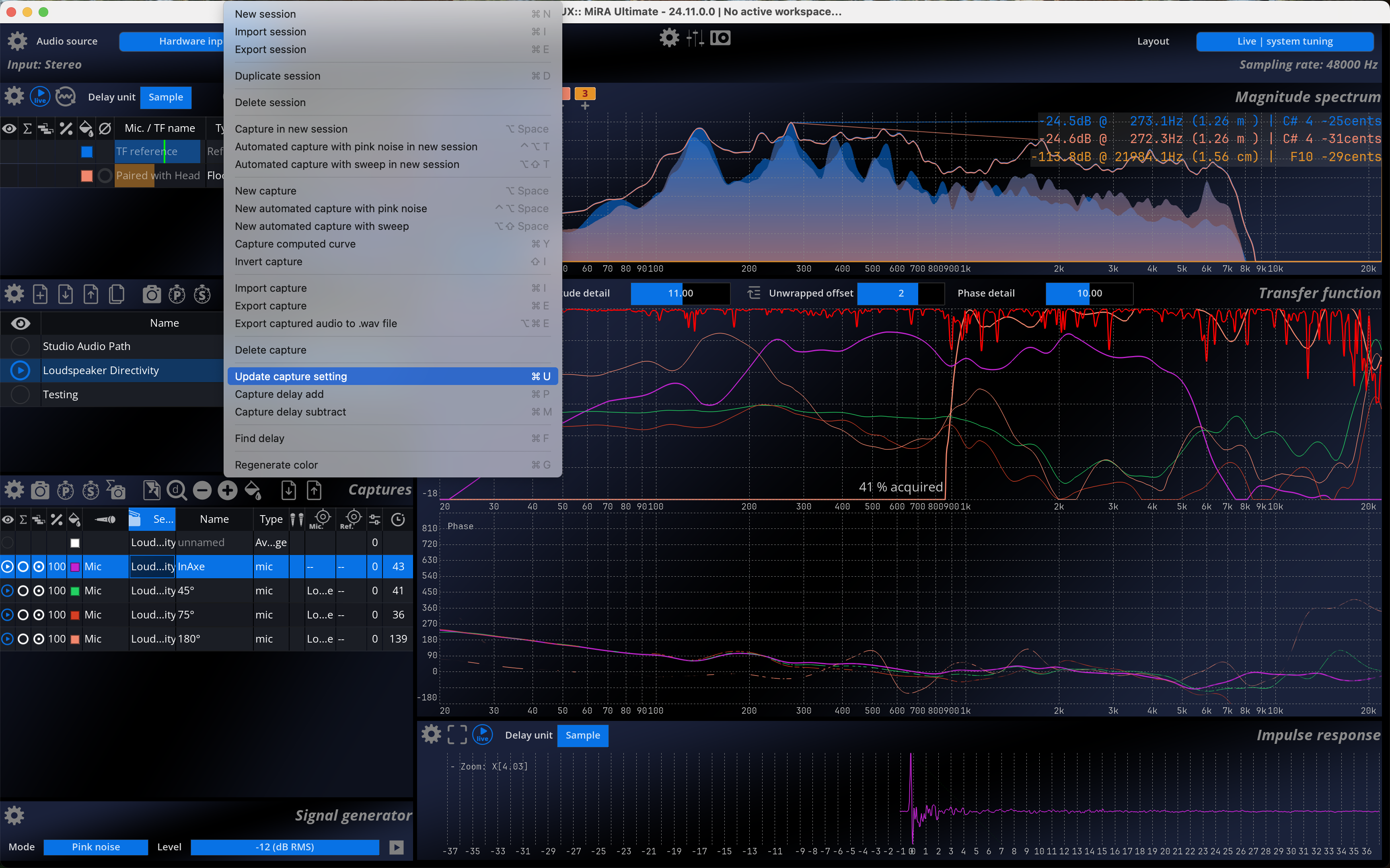
By default, newly created captures follow the settings of the transfer function. If you want to change the spectrum type, block size or time averaging afterwards, you can use the “Update capture setting” option in the “Capture” menu in the top menu of the application.