Main Setup
The Main Setup section allows you to configure various aspects of the application, including saving and restoring user-defined configurations, setting up the SampleGrabber password for secure audio material access, specifying graphic engine frame rates, adjusting timecode settings, and configuring main analysis parameters such as RTA block size, spectrum type, TF/Sweep block size, overlap mode, analysis window, normalization, scaling, and averaging. Additionally, you can set various preferences, like the auto-pause threshold, metric system, temperature, and reset preferences to their default values. Each setting is designed to optimize the performance and usability of the application based on your specific needs.
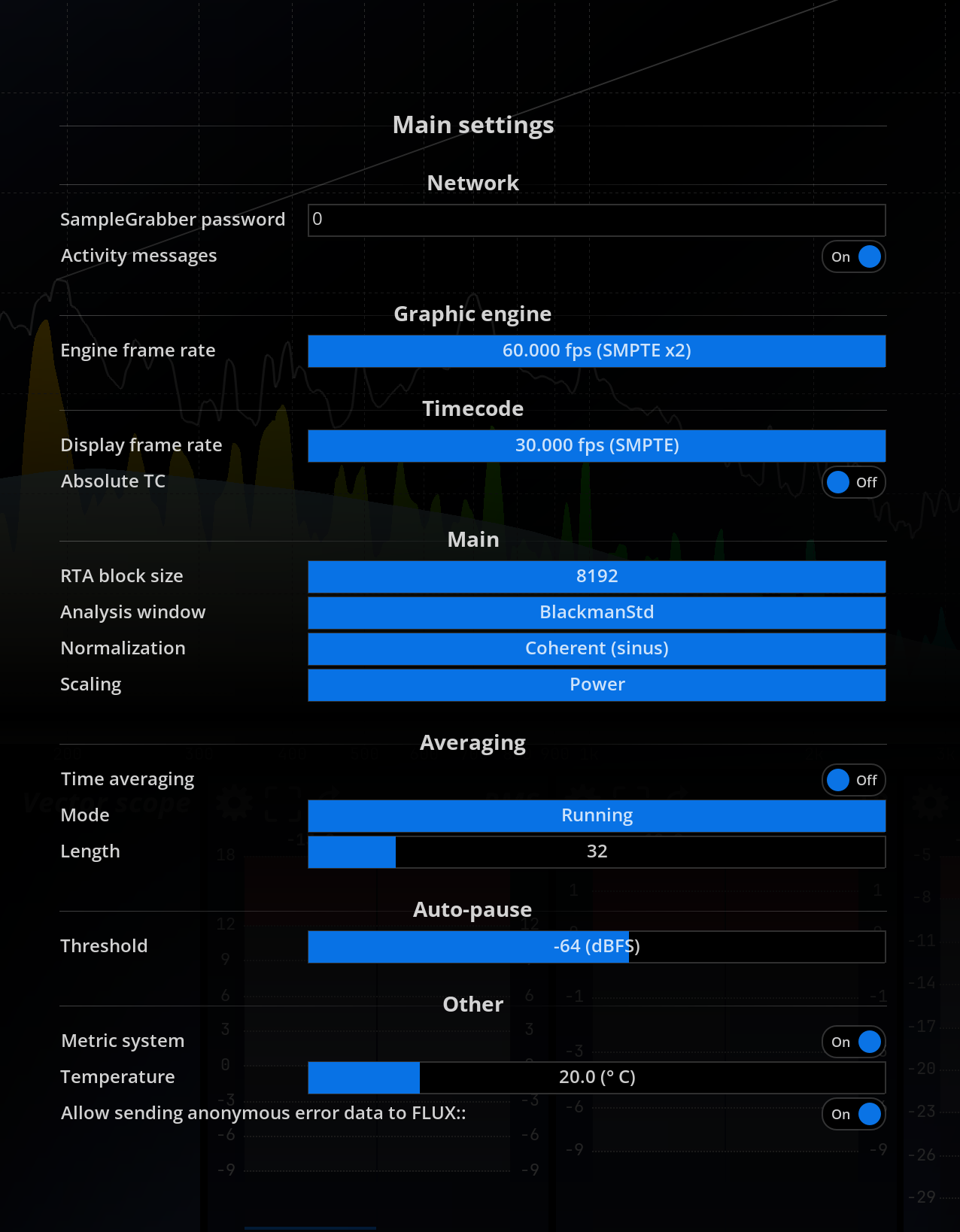
Main setup dialog
Configuration
Save/restore a user-defined configuration to and from disk, including all the settings in this panel, as well as IO Configuration IO Configuration and UI Setup UI Setup.
SampleGrabber
SampleGrabber password
The password entered in this field should match the one used by the SampleGrabber you wish to use as a source. This provides a reasonable level of security and prevents unauthorized access to your audio material broadcast over the network. Please consider that the encryption used only provides moderate protection, and is not intended to replace other security guards, such as firewalls, etc.
Graphic engine
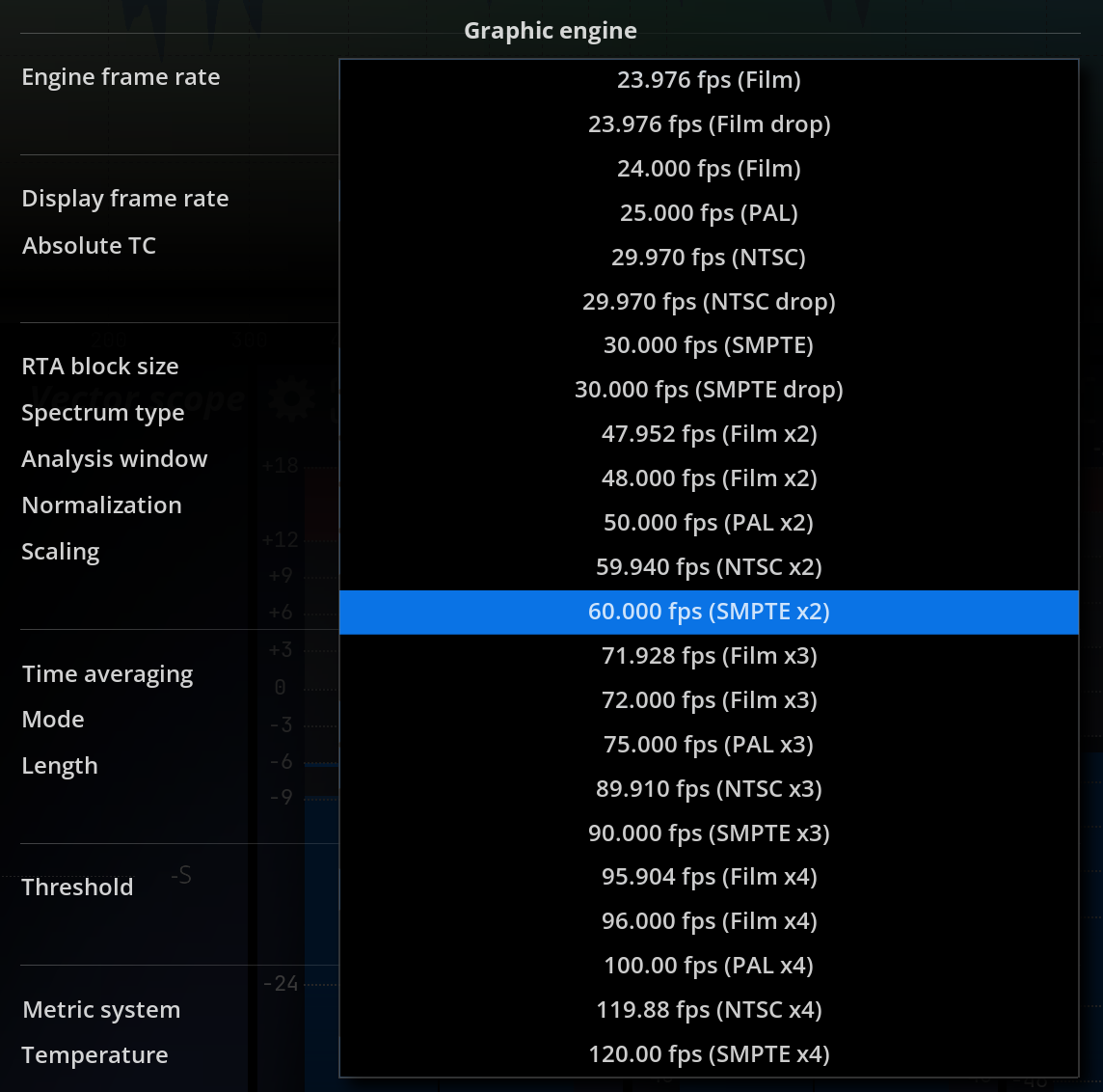
Available graphic engine frame rates
Here, you can specify the rate at which the display should be refreshed. Please note higher frame rates place higher demands on the GPU, and, to a lesser extent, on the CPU.
The effective frame rate can be displayed by typing
SetRenderStats(1)in the console.
Timecode
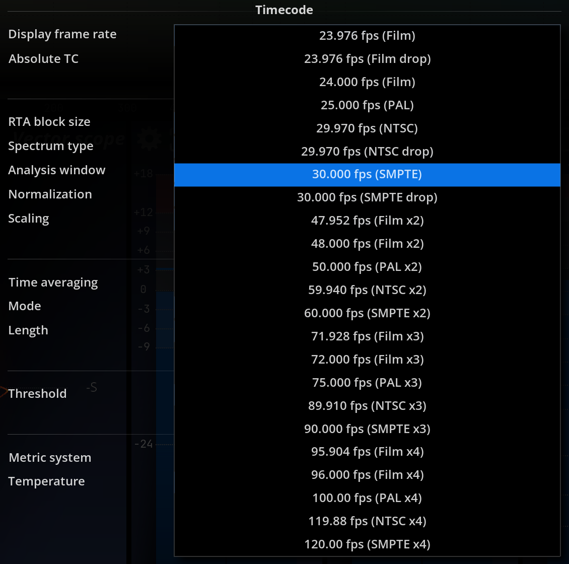
Display frame rate
Sets the frame rate used for time display in various parts of the program. Set it to match the frame rate of your source material to facilitate locating time events when working with film, TV or other time-stamped material.
Absolute Timecode
This setting toggles between absolute and relative time-code display formats. Absolute Timecode is taken from the time the application was started. Relative Timecode is the time-elapsed since the Timecode offset position. See metering history usage Usage for information on working with Timecode.
Main
RTA block size
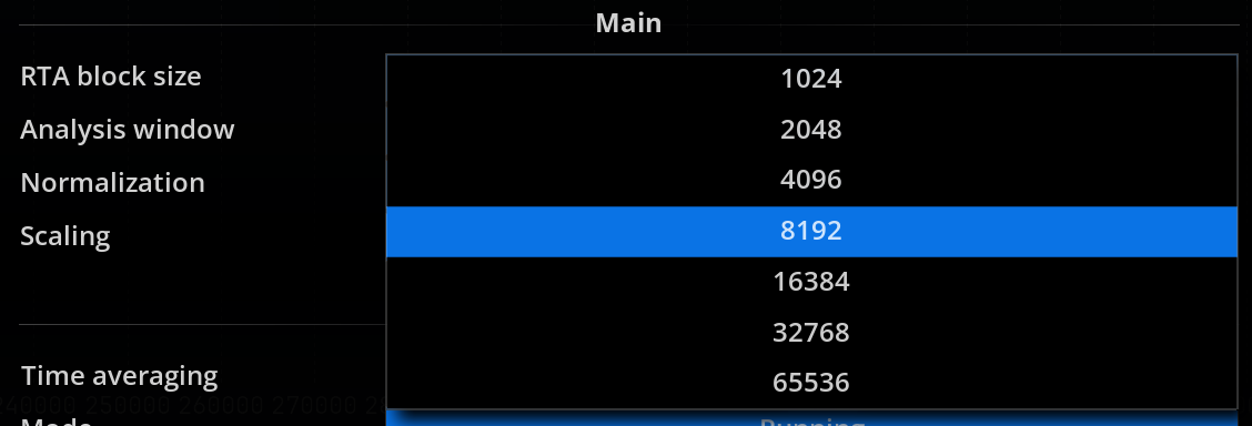
Defines the size of the blocks in samples, fed to the main spectrum analyzer engine, which is used by the spectrum magnitude, Nebula and spectrogram views.
Keep in mind that the incoming audio needs to be accumulated in a buffer for a certain amount of time before the data can be computed and the display updated. In contrast with the buffers you probably know from sound cards, this block processing is not just a computer technicality nor a source of undesirable latency, but an integral part of the analysis process.
As such, it determines both the precision of the analysis and the maximum display rate, and should be adjusted depending on the specifics of your application.
In order to maintain a sufficiently responsive display refresh rate, blocks overlap by 75 %.
The default setting is 8192 samples, corresponding to a length of roughly 180ms at 44.1kHz sampling rate. This value constitutes a good compromise between precision and responsiveness for most situations. However, if you need to measure a particular frequency with great precision, you should raise the analysis block size. On the other hand, if you need to follow rapid spectrum variations, this value should be lowered.
Analysis window
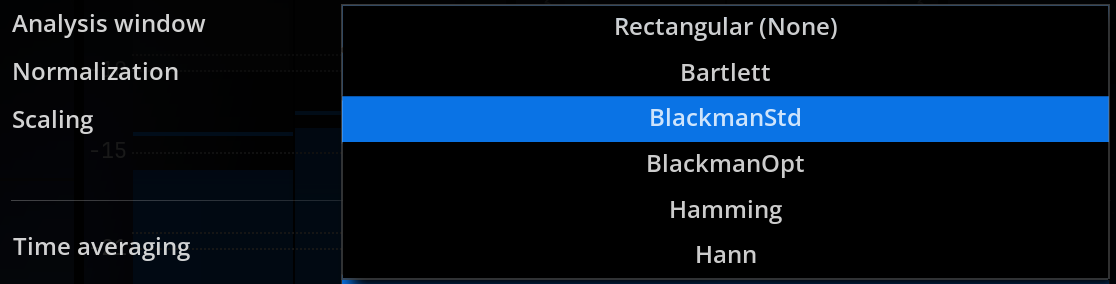
The first step of signal analysis is to split the incoming signal into overlapping blocks. Each block is then multiplied with a so-called window signal prior to the spectrum computation. The purpose of this is to minimize the side effects of block processing, such as the introduction of transients at the block boundaries, etc.
Available choices are:
- Rectangular (None).
- Bartlett.
- Blackmann standard (default).
- Blackmann optimized.
- Hamming.
- Hann.
We suggest you leave this setting to the default unless you are quite knowledgeable about these aspects, or if you should need to explicitly recreate a specific measurement, such as a particular method specified in a standard document.
Normalization

Selects the normalization mode used to normalize the global gain of the spectrum display.
Available choices are:
- Coherent (sinus): 0dB peak sine gives 0dB amplitude.
- Incoherent (noise/music): 0dB RMS noise or music gives 0dB power.
Scaling

This setting controls the frequency dependent amplitude spectrum correction curve.
This affects how various standard reference signals register on the display. The default power scaling will result in a signal with spectrum components of constant power registering as a flat curve, whilst amplitude will have the same effect for components of constant amplitude such as pure tones (sine signal).
The table below shows how the curve appears depending on the type of input signal. 1/f corresponds to a rectilinear slope on the display with both X and Y axis being logarithmic.
| Input signal | Sine | White | Pink noise |
|---|---|---|---|
| Power scaling | 1/f | 1/f | Flat |
| Amplitude scaling | Flat | Flat | 1/f |
For monitoring a mix, it makes the most sense to use power scaling, as this is the way our hearing responds. If you need to measure a room’s acoustic response, an outboard unit or a plugin’s frequency response, the system’s magnitude transfer function is best suited for this purpose and scaling has no effect.
The amplitude scaling setting should therefore really be employed if you need to measure relative amplitude values, such as those of sine test tones at various frequencies. Also, note that plain DFT corresponds to scaling set to amplitude.
The power of a time signal is proportional to the square of its amplitude, or equivalently, its power in dB is double the amplitude. However, in the case of a spectrum, we are measuring the output of a filter bank, which reacts very much differently depending on the type of input signal, so the simple previous formula doesn’t apply anymore.
Available choices are:
Amplitude: equivalent to no scaling. The amplitude of pure tones at different frequencies registers at the same value. Incoming white noise is displayed as a (quasi) flat curve.
Power (default): scaling inversely proportional to frequency (1/f). Incoming pink noise is displayed as a flat curve.
Averaging

Time averaging: engages averaging of spectrum magnitudes over time. Default is off.
Mode
Running: the average display is updated as soon as a new incoming block arrives. This is the default.
Fill-freeze: the display is only updated when a fresh batch of N new incoming blocks has arrived. The display is frozen until the next batch of N blocks arrives, and so on. N corresponds to the length setting defined below.
Length
The number of incoming blocks over which the resulting average spectrum is computed. Lower values lead to faster apparent display update rates, while higher values smooth-out any time-variations more. Default is 32.
Running average employs a weighting window that gives more importance to the last incoming blocks of samples. This type of time averaging is also called moving average, rolling average or running average, and is good for smoothing out abrupt variations in time and still be able to monitor in a continuous fashion.
Fill-freeze mode is useful for stabilizing a flickering display while still following long-term variations, which permits a more detailed study of the curve(s). This mode is therefore useful to get a very steady picture of the spectrum while still monitoring some of the mid-term changes, and saves you from holding and resetting the display manually again and again.
Various
Auto-pause threshold
Analysis is paused whenever the level of any channel of the incoming audio falls below this level. Set this a tad above the acoustic and electronic noise floor of your input signal chain to retain measurements even though the audio (music program or test signal) has stopped.
Metric system
Toggle displayed units between:
- Metric system (default): distance expressed in meters, temperature in degrees Celsius.
- Imperial units: distance expressed in inches and feet, temperature in degrees Fahrenheit.
Temperature
This should be set to the ambient temperature at the current location in order to get the most accurate time to distance conversions in the delay finder and impulse response panels. The following table gives an idea of how much the speed of sound varies with temperature.
| Temperature (°C) | Speed of sound (m/s) |
|---|---|
| 0 | 331.3 |
| 15 | 340.31 |
| 25 | 346.18 |
| 35 | 351.96 |
Allow sending anonymous error data to FLUX
Allow sending error data to FLUX:: support. All the data are sent anonymously.