System Setup
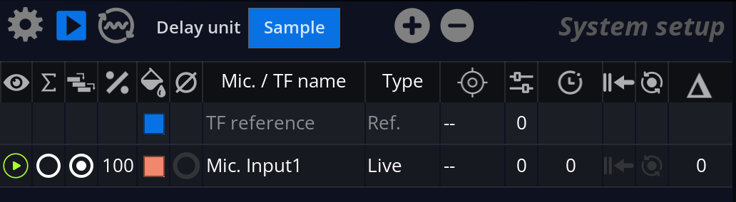
The system setup UI scope lists all the inputs from the live system, along with their associated options. Here, you will be able to name the input, compensate for delay offsets, apply a target reference, associate a floor and a head microphone, etc. Each input gives four curves:
To these curve, it’s possible to associate an EQ curve. This EQ curve can be computed using the Auto-EQ feature, or manually edited using the scope. More information on the EQ page.
Basic operations
The visibility of an input is defined by the toggle in the ![]() column.
column.
To rename an input, double-click on its name in the ‘Mic./TF name’ column.
To change the color, double-click on the colored square in the ![]() column.
column.
Gain and target
The ![]() column allows for adjustment of the gain of each capture, in decibels.
column allows for adjustment of the gain of each capture, in decibels.
The ![]() button toggles phase inversion of the selected channel.
button toggles phase inversion of the selected channel.
A reference target for the input can be defined in the ![]() column.A target is a previously recorded capture that is used as a reference for the input. For example, it is often used to calibrate measurement microphones.
column.A target is a previously recorded capture that is used as a reference for the input. For example, it is often used to calibrate measurement microphones.
Computed Curve
The computed curve appears automatically in the system setup list if more than one microphone is present. To feed an input into the computed curve, you must check its \(\sum\) column.
Several computed curves can be added to the system setup or to a session. They are named “Computed 1”, “Computed 2”, etc. They can be added using the action “Add computed curve” in the System Setup menu, or “Add computed capture curve” in the Capture menu.
When several captures are available, several  appears, the color matching the computed curve one.
The computed curve has four different computing algorithms, which can be accessed in the “type” column.
- The averaging mode is recommended when using several microphones at different locations in the same venue. When using this algorithm, you can adjust the weight of a microphone by adjusting the \(\%\) column. One hundred percent indicates full contribution, while zero percent indicates no contribution. The coherence score also affects the computed curve: a measure with low coherence will have its weight lowered. You can deactivate this behavior by unchecking the combo box in the
 column.
 - The sum mode simply adds the magnitudes of the different curves.
- The acoustic mode summarizes the magnitude, but it also takes phase relationships into account. This mode is recommended when dealing with separated measurements for heads and sub speakers.
- The max mode keeps the highest magnitude value per analysis band among contributing captures.
Choosing a computed curve mode
| Situation | Recommended mode | Why |
|---|---|---|
| Several microphones covering the same listening area | Averaging | Gives a practical spatial average and can reduce the influence of low-coherence measurements. |
| Combining separated sources such as heads and subs | Acoustic mode | Takes phase relationships into account, so it is better suited to crossover and summation decisions. |
| Comparing coverage and worst-case tonal balance | Max | Shows the highest magnitude found per band, useful for checking zones that may become too loud after EQ. |
| Technical checks where simple level addition is required | Sum | Adds magnitudes directly and is mainly useful for controlled diagnostic cases. |
Start with Averaging for general system EQ decisions, then check Max before exporting corrections if the venue has very uneven coverage. Use Acoustic mode when the question is about source interaction rather than tonal average.
The computed curve is not a capture. It is a virtual curve that is computed on the fly from the available captures. For live computed curves, phase and coherence are not provided as dedicated computed traces.
You can have up to 4 live computed curves. The first one will be automatically added when adding a second microphone. The other ones can be added using the action “Add computed curve” in the “System setup” menu.
Delay finder
FLUX:: MiRA uses an automatic delay-finding algorithm to determine the time-of-arrival difference between several microphones and the reference input.
The delay unit can be chosen from the drop-down menu. Possible options are:
- Delay in samples (smp).
- Distance in meters (m) or imperial feet (ft.).
- Delay in milliseconds (ms).
The delay finder always tracks for delay changes. The detected offset is displayed in the \(\Delta\) column in red.
Delay compensation
Pressing the ![]() button activates a delay line in the source signal path, compensating for the currently displayed delay value. This effectively aligns the source and response signals.
button activates a delay line in the source signal path, compensating for the currently displayed delay value. This effectively aligns the source and response signals.
If necessary, you can manually adjust the delay figure using either of these methods:
- Direct keyboard numeric value entry as time or distance figure.
- Increment / decrement by clicking the +/- icons.
- Increment / decrement using the +/- numeric keys.
Delay adjustment considerations
Ensure stable conditions while performing a measurement
You should ensure both source and response signals have reached stability before attempting measurement. In particular, do not stop or start the audio, change the volume or any other parameter just before or during measurement. This would invalidate the measurement and you would have to start again.
Limitations
Please note there are many unknowns in play when determining the optimum delay figure. While we did our best to make this tool as robust and accurate as possible, there is always a possibility that it will fail, as with all automatic procedures. In this case, you should repeat the process or resort to manual adjustment until you get satisfactory results.
Multiple Paths
The major assumption behind delay compensation is that there is a main direct path from source to listener. This obviously does not apply in a very reverberant or complex-shaped acoustic space. This is where acoustic expertise and trial and error come into play in order to attain the best compromise.
Input Type
An input microphone can be of three different types. By default it is considered as a “Live (full band)” input.
The other accessible type is “Live Floor Mic (pair with..)”. When a microphone is switched to this type, it is expected to be placed on the floor to reduce the influence of floor reflections in the measurement process. It is then paired with another microphone. The one on the ground will produce data for the low frequency content of the measure, while the paired microphone will produce the data for the high frequency content. The crossover between the two microphones can be set in the configuration menus of the system setup.
The pairing algorithm can be selected per input. Available modes are Crossover, Coherence max., Weighted average, and Hybrid.
The reference input displays a type of “Ref.” and cannot be edited.
The computation curve uses the type to define its averaging algorithm. See the section above.
Header buttons

For common scope header buttons, see the Audio Analysis Scopes section.
When the ![]() is engaged, it loops the first output channel of the signal generator into the reference input of the system setup. This setting is also accessible from the IO configuration menu.
is engaged, it loops the first output channel of the signal generator into the reference input of the system setup. This setting is also accessible from the IO configuration menu.
The “Delay unit” drop-down allows for changing the delay unit, as seen in the delay finder section above. The ![]()
![]() buttons allows for changing the delay value of the selected input by \(\pm\) 1 sample.
buttons allows for changing the delay value of the selected input by \(\pm\) 1 sample.
Options menu
The options menu is accessible by clicking on the ![]() button.
button.
The Delay Finder FIFO parameter sets both the maximum delay time that can be found as well as the global time averaging of the delay finder. It can most often be left to its default setting.
History time defines the length of the analysis buffer. It is set to 5 seconds by default, and can be adjusted between 1 and 15 seconds.
Pairing crossover freq. sets the crossover point for floor/head microphone pairs (100 Hz to 22 kHz, default 1 kHz).
Auto-pause: when the signal is below the level indicated on the Main IO, the Transfer Function will not be processed. Default threshold is -64 dBFS.
Columns visibility allows you to show/hide specific table settings.