Transfer function
Introduction
The transfer function of a system measures its frequency response, which is expressed in terms of magnitude and phase response. The transfer function measures how the system affects the magnitude and phase of an incoming signal at different frequencies, and is essentially a ratio of output versus input spectra.
Practical uses of this are numerous: determining the curve of an equalizer, determining what frequencies are emphasized by an outboard device, measuring a room’s acoustic response, etc.
The transfer function assumes the system is linear and time-invariant. Linearity notably implies the system is free of distortion, and time invariance that its characteristics do not change in time. Failing to meet these requirements will lead to unpredictable results.
In practice, the transfer function is considered an adequate measurement technique for most real-world systems, except for devices exhibiting highly non-linear behavior, such as compressors and distortion effects, and time-modulation based effects, such as chorus and flanger.
Transfer function magnitude
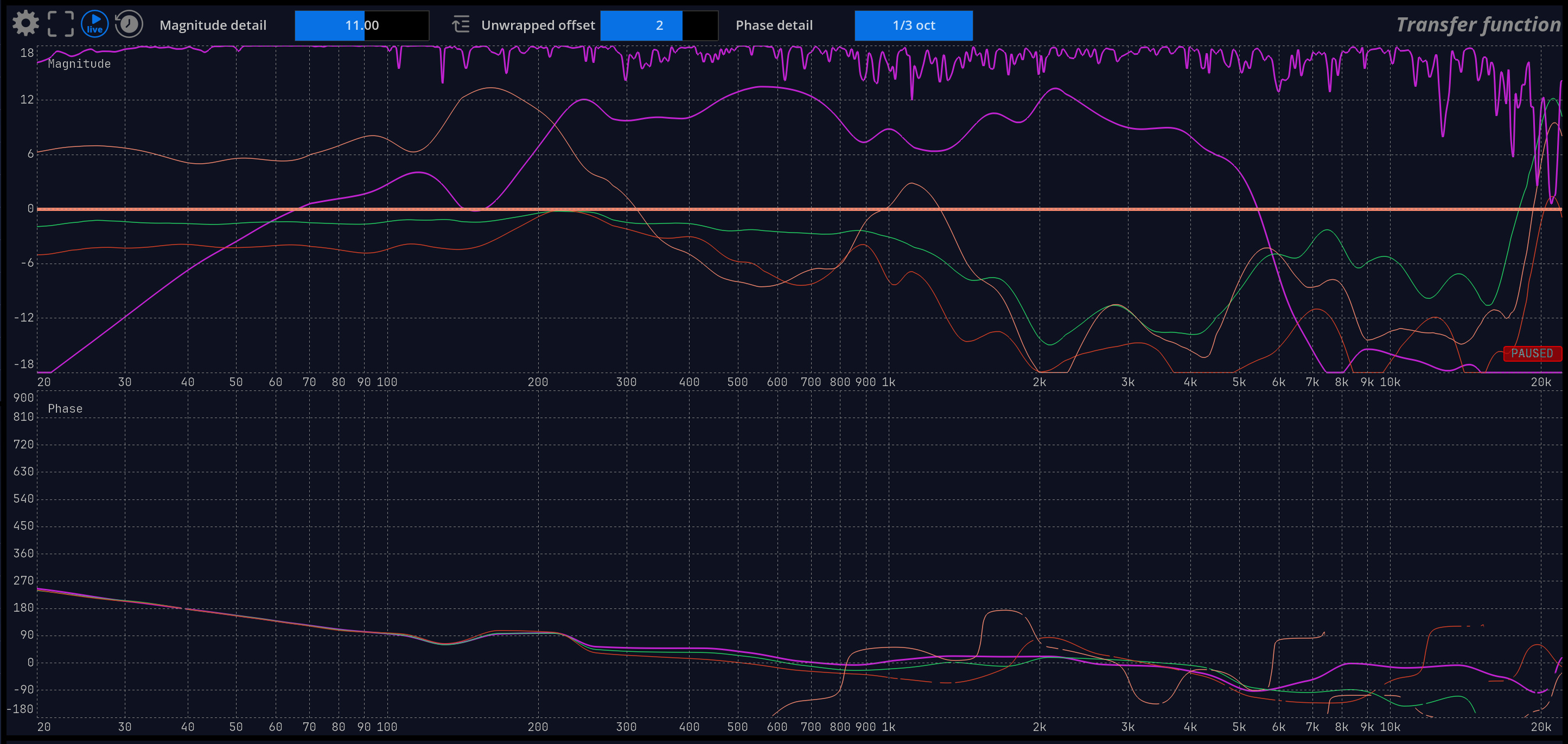
The transfer function magnitude displays the gain versus frequency curve of the system under test. A passthrough obviously results in a flat horizontal line centered on 0dB. This line represents the ideal curve one would be able to achieve if all the system defects could be compensated for, and that serves as a reference target when doing room correction.
Transfer function coherence
The coherence is a normalized - that is comprised between zero and one - measure of the confidence of the transfer function at a specific frequency. In other words, it describes how trustworthy the transfer function is at the corresponding frequency.
Coherence at a particular frequency indicates whether the system can accurately be described as linear gain and phase shift or not.
Interpretation and uses
A low coherence most often indicates a bad measurement, so you should look for possible causes and correct them before starting again. Improper delay compensation leads to low coherence results, so this is the first thing to check. Other typical culprits include a noisy device, the presence of distortion, channel crosstalk, acoustical noise such as cooling fans, people talking, handling noise, bad isolation from the outside, etc.
While maximizing the coherence is desirable, in most cases, it will most likely be impossible to attain a flat curve approaching unity at all frequencies, except in an anechoic chamber or very ‘dead’ sounding room with minimal reflections.
Reverberation, as well as mismatched transducers, tend to give lower coherence, as the signal arriving at the microphone position is really the sum of several time-delayed versions of the source.
Sometimes, it will be impossible to get good overall coherence, and the magnitude and phase curves will, therefore, be less precise, stable and smooth. This does not mean you cannot attempt to extract any information from those. As always, use your judgment and knowledge of the specific system to decide which assumptions seem reasonable.
Transfer function phase
Phase information is sometimes overlooked, and indeed it is less straightforward to understand and interpret than magnitude. Altering the phase of a signal can range from subtle to dramatic, and phase distortion can lead to temporal smearing of the audio, loss of spatial information, and other nuisances.
The transfer function phase curve displays the phase difference between the system’s output and input at different frequencies, in degrees, ranging from -180 to 180.
FLUX:: MiRA employs several smoothing algorithms custom designed for phase curve smoothing, as explained in the section about phase setup.
Due to the definition of phase itself and the means of computing it, the curve is generally more sensitive to extraneous noise, distortion and time-varying conditions.
Even more so than with the magnitude curve, a precisely compensated delay is critical to accurate phase computation. In very reverberant environments, the phase curve will be very chaotic. This is inevitable and a direct consequence of the complex nature of the system, and not a limitation of the instrument.
We advise using ART analysis mode, which mitigates phase computation inaccuracies compared to plain FFT.
Settings
Time averaging is on by default, as the goal here is to provide the most stable display, and to eliminate any variations of the signal in time.
Frequency smoothing can be useful to smooth out irregularities and get a general picture of the curve. It is advised to use this function sparingly, though, as it can change values by a large proportion, and obscure potential problems with either the actual system being measured, or the measurement setup itself.
A combination of time averaging and frequency smoothing is most often required to obtain readable results in real-world scenarios, especially in large rooms and outdoors.
Main
| Name | Description |
|---|---|
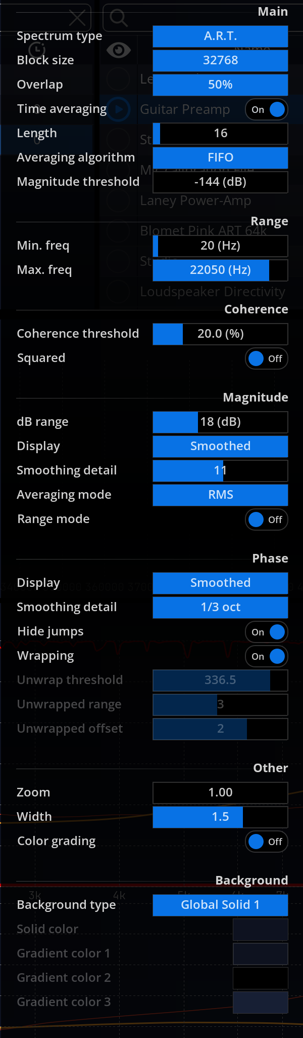
| Block size | Block size used for the transfer function and the capture done with sweep. The default is 65536, which is appropriate for most cases. Increasing this value gives better frequency resolution, at the expense of CPU load. Lower values can be employed if you’re only interested in the overall response of the analyzed system. 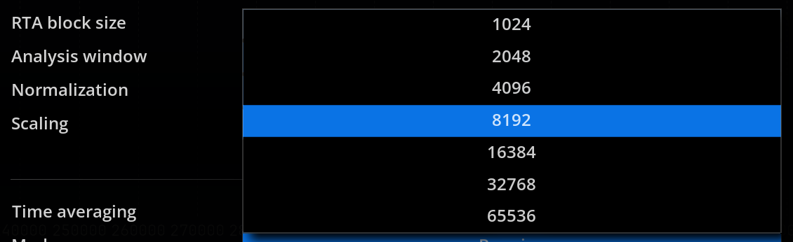 |
| Overlap | The overlap mode setting determines how much incoming audio frames overlap each-other. A higher overlap results in a smoother display update, at the expense of increased CPU usage. The available settings are: 85%: highest overlap 75%: medium overlap size. 50%: minimized overlap for minimal CPU usage (useful for slow machines) 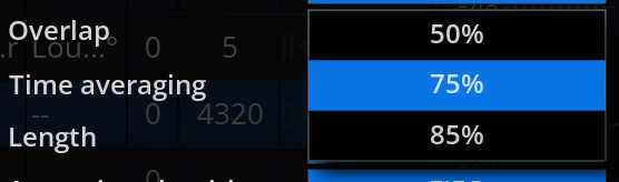 |
| Time averaging | Toggles time averaging on and off. Default is on, which, in most cases, is necessary to provide a stable display readout. |
| Length | This setting determines the number of blocks that are taken into account to compute the averaged transfer function. Increasing this value will give a smoother readout, but the display will react more slowly to any input variations, and CPU load and memory consumption will be higher. The default is 32. |
| Averaging algorithm | Averaging can be performed using two different algorithms: - The FIFO mode (First-In First-Out) corresponds to a simple sliding averaging. - The exponential mode is equivalent to a first order low-pass filter. |
| Magnitude threshold | Set the detection level of each frequency bin displayed in the transfer function. When the level of a frequency bin is below this threshold, the signal is effectively gated. This mechanism ensures a better measurement and increases the coherence. When a frequency bin is gated, a red line at the bottom of the transfer function is displayed. |
Be aware that the auto-pause settings from the system setup scope also interact with the magnitude threshold setting of the transfer function. The signal is firstly gated by the auto-pause feature, then by the magnitude threshold. The magnitude threshold should be therefore always be set above the auto-pause threshold.
Range
| Name | Description |
|---|---|
| Min. Freq | Minimum frequency display by the transfer function |
| Max. Freq | Maximum frequency display by the transfer function |
Coherence/magnitude
| Name | Description |
|---|---|
| Smoothing detail | Sets the amount of detail present on the smoothed magnitude and coherence curves. This number is roughly the maximum number of valleys and peaks that will remain after smoothing. A low value of around 10 is good for getting a global and uncluttered picture of a room’s frequency response. 1 |
Coherence
| Name | Description |
|---|---|
| Squared | Apply a square function to the coherence values. |
| Display | Toggles between one of three modes: - Full: raw coherence curve. - Smoothed: smoothed coherence only. - All: both.  |
| Color | Color of the pen used to draw the coherence curve. |
Magnitude
| Name | Description |
|---|---|
| Range | Minimum and maximum values to which the display is clamped, in decibels. |
| Display | Toggles between various combinations of raw and smoothed magnitude curve display. 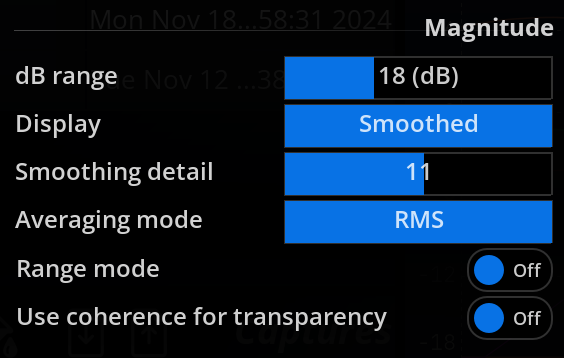 - Full : raw magnitude curve. - Smoothed: smoothed magnitude only. - All: both. Keep in mind the smoothing process can filter out a lot of information, so relying solely on the smoothed curve should be avoided. |
| Smoothing detail | Adjust the amount of detail displayed in the curve. Lower values imply more smoothing. This setting should be set so that the curve shows meaningful and accurate information. Too little details will induce a loss of information, while too many details will display information that may be inaccurate. |
| Averaging mode | Choose the averaging mode of the transfer function magnitude. Vectorial mode computes the average sum of magnitudes and magnitudes multiplied by coherence. In vectorial mode, the averaged magnitude is therefore an indication of the perceived magnitude spectrum, i.e. the sum of the direct path and diffuse field signals. RMS mode computes the average as the root of the sum of the square magnitudes. Default is RMS. |
| Range mode | Toggles auto-range on and off. When enabled, the display range automatically follows that of the transfer function magnitude curves, which is useful for hands-free operation, for example. Default is off. |
| Use coherence for transparency | Allows to use the coherence values to define Magnitude. |
Phase
| Name | Description |
|---|---|
| Display | Toggles between the various phase curve display modes: - Full: raw phase only. - Smoothed: smoothed phase only. - All: both. |
| Smoothing detail | Adjust the amount of detail displayed in the curve. The widest fractional octave values give a smoother curve. This setting should be set so that the curve shows meaningful and accurate information. Too little details will induce a loss of information, while too many details will display information that may be inaccurate. |
| Coherence threshold | Mask phase curve region where the coherence is below this threshold |
| Unwrap threshold | Raise to unwrap larger phase jumps only (only relevant in tolerance mode) |
| Hide jumps | When enabled, the portion of the curve that corresponds to a phase rotation is not displayed. |
| Wrapping | Display the phase either wrapped between -180° and 180° or unwrapped. |
| Unwrapped range | Adjust the phase range, for \(-n \times 180\) to \(n \times 180\), where \(n\) is the value of this settings. |
| Unwrapped offset | Increment an offset of \(n \times 180°\), where \(n\) is the value of this settings. |
Other
| Name | Description |
|---|---|
| Color grading | Apply frequency-dependent coloring to the curve. Default is off. |
| Zoom | Curve zoom ratio slider. |
| Width | Size of the pen used to draw the coherence curve. |
Relying on smoothed curves altogether should be avoided, as smoothing can mask-out essential information such as room modes, which materialize as sharp peaks and dips in the transfer function magnitude curve.
We strongly recommend basing your judgment on both raw and smoothed curves even when the raw curve is very noisy.↩︎